Partial-Least Square SEM (PLS-SEM)
1 Sample study
- Journal article: Young people’s perceived service quality and environmental performance of hybrid electric bus.
- Author: Zial Haque and Tehjeeb Noor
- Article link: DOI link
- Download the dataset here
2 Libraries
# Library
library(tidyverse)
library(readxl)
library(janitor)
library(seminr)
library(psych)
library(MVN)
library(semTools)
3 Data
## data
case_data <- read_excel("00_data/e_bus_customer_satisfaction.xlsx") %>%
 clean_names()

case_data_items <- case_data %>%
 select(bt1:bt7, bd1:bd4, emp1:emp5, cs1:cs3, ep1:ep4, ls1:ls5)
4 Exploratory factor analysis
4.1 Scree plot
## Scree plot using parallel analysis
fa.parallel(case_data_items, fa = "fa")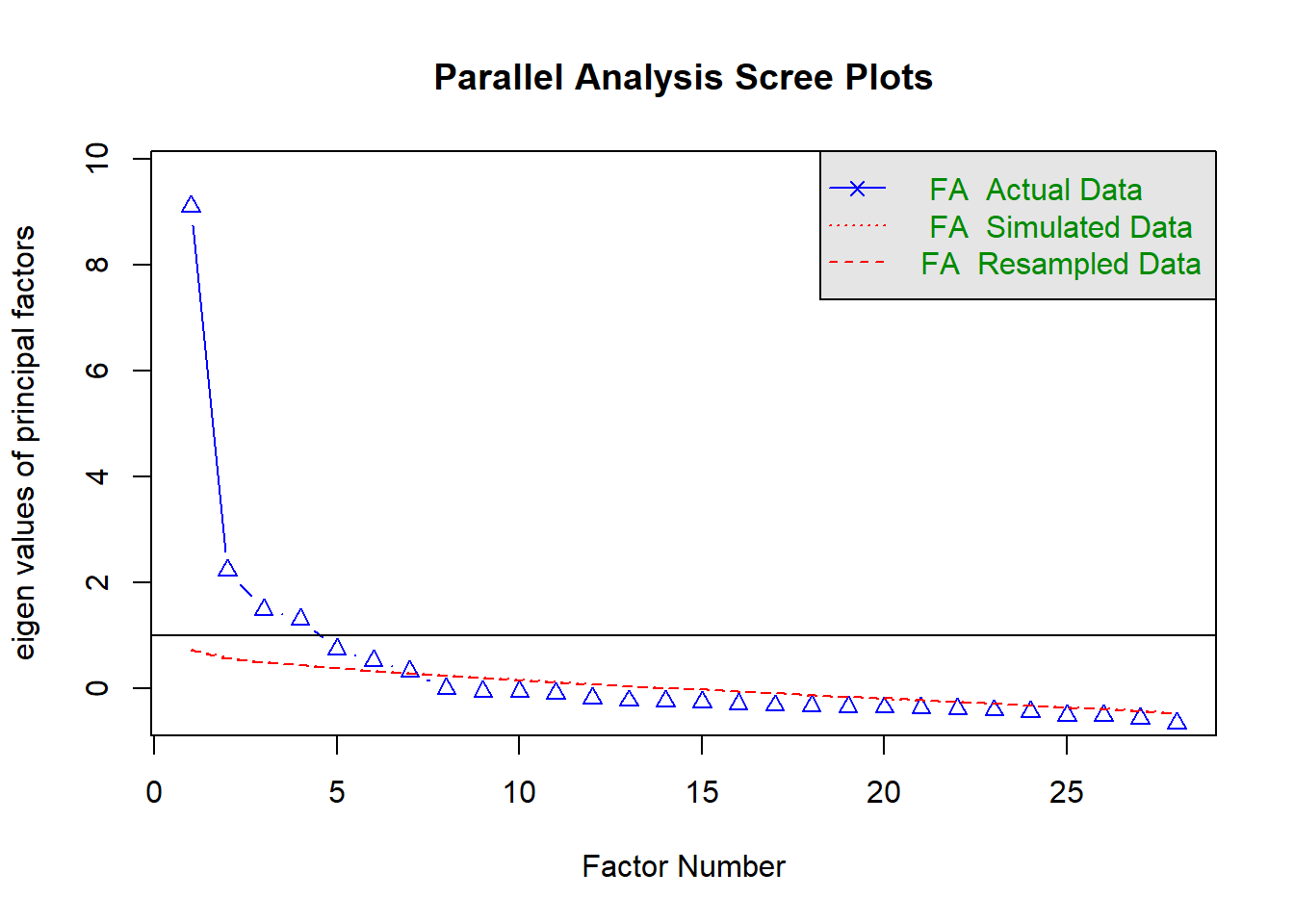
Parallel analysis suggests that the number of factors = 7 and the number of components = NA 4.2 Factor extraction
## Factor loading
bus_fa <- fa(r = case_data_items,
             nfactors = 6,
             rotate = "varimax")

print(bus_fa$loadings, sort = TRUE, cutoff = 0.4)
Loadings:
     MR2   MR1   MR3   MR4   MR6   MR5
ls1  0.820
ls2  0.891
ls3  0.828
ls4  0.806
ls5  0.599
bt1        0.673
bt2        0.666
bt4        0.549
bt5        0.680
bt6        0.578
bt7        0.550
ep1              0.864
ep2              0.900
ep3              0.690
ep4              0.705
emp1                   0.688
emp2                   0.662
emp3                   0.636
emp4                   0.697
emp5                   0.502
bd1                          0.679
bd2                          0.640
bd3                          0.676
bd4                          0.629
cs1                                0.774
cs2                                0.817
cs3                                0.768
bt3        0.476

                 MR2   MR1   MR3   MR4   MR6   MR5
SS loadings    3.477 3.363 3.081 2.658 2.429 2.297
Proportion Var 0.124 0.120 0.110 0.095 0.087 0.082
Cumulative Var 0.124 0.244 0.354 0.449 0.536 0.618
5 Partial-least square SEM
5.1 Specifying the measurement model
pls_mm_ebus <-
  constructs(
  composite("tangible", multi_items("bt", c(1:2, 5:7))),
  composite("drivers_quality", multi_items("bd", 1:4)),
  composite("empathy", multi_items("emp", 1:5)),
  composite("env_perf", multi_items("ep", 1:4)),
  composite("customer_sat", multi_items("cs", 1:3)),
  composite("life_sat", multi_items("ls", 1:5))
)

plot(pls_mm_ebus)
5.2 Specifying the structural model
pls_sm_ebus <-
  relationships(
  paths(from = c("tangible", "drivers_quality", "empathy", "env_perf"),
        to = "customer_sat"),
  paths(from = "customer_sat", to = "life_sat")
)

plot(pls_sm_ebus)
5.3 Estimating PLS-SEM model
pls_model_ebus <-
  estimate_pls(
  data = case_data,
  measurement_model = pls_mm_ebus,
  structural_model = pls_sm_ebus
)


plot(pls_model_ebus)
summary_pls_model_ebus <- summary(pls_model_ebus)
summary_pls_model_ebus
Results from  package seminr (2.3.2)

Path Coefficients:
                customer_sat life_sat
R^2                    0.448    0.077
AdjR^2                 0.440    0.074
tangible               0.179        .
drivers_quality        0.146        .
empathy                0.310        .
env_perf               0.237        .
customer_sat               .    0.278

Reliability:
                alpha  rhoC   AVE  rhoA
tangible        0.830 0.880 0.595 0.831
drivers_quality 0.856 0.902 0.698 0.857
empathy         0.825 0.876 0.586 0.840
env_perf        0.920 0.944 0.808 0.926
customer_sat    0.941 0.962 0.895 0.944
life_sat        0.903 0.929 0.724 0.911

Alpha, rhoC, and rhoA should exceed 0.7 while AVE should exceed 0.5
5.4 Bootstraping PLS-SEM
## bootstrapping PLS-SEM model
boot_pls_model_ebus <- bootstrap_model(seminr_model = pls_model_ebus,
                nboot = 1000)

## summary results
summary_boot_pls_model_ebus <- summary(boot_pls_model_ebus, alpha = 0.10)
5.5 Factor loadings
# DT::datatable(summary_boot_pls_model_ebus$bootstrapped_loadings %>% round(3))
summary_boot_pls_model_ebus$bootstrapped_loadings
Original Est. Bootstrap Mean Bootstrap SD T Stat.
bt1 -> tangible 0.763 0.761 0.036 21.496
bt2 -> tangible 0.766 0.764 0.035 21.673
bt5 -> tangible 0.767 0.766 0.032 24.108
bt6 -> tangible 0.790 0.787 0.030 26.736
bt7 -> tangible 0.772 0.770 0.034 22.580
bd1 -> drivers_quality 0.834 0.834 0.021 40.400
bd2 -> drivers_quality 0.823 0.821 0.024 34.655
bd3 -> drivers_quality 0.858 0.857 0.018 48.626
bd4 -> drivers_quality 0.826 0.825 0.026 31.977
emp1 -> empathy 0.768 0.766 0.030 25.914
emp2 -> empathy 0.799 0.797 0.026 30.163
emp3 -> empathy 0.699 0.696 0.041 17.024
emp4 -> empathy 0.794 0.792 0.029 26.930
emp5 -> empathy 0.762 0.762 0.029 26.369
ep1 -> env_perf 0.905 0.903 0.019 47.944
ep2 -> env_perf 0.947 0.946 0.010 99.625
ep3 -> env_perf 0.875 0.877 0.020 43.729
ep4 -> env_perf 0.866 0.866 0.028 31.239
cs1 -> customer_sat 0.944 0.944 0.012 79.744
cs2 -> customer_sat 0.960 0.960 0.007 142.935
cs3 -> customer_sat 0.934 0.933 0.015 60.711
ls1 -> life_sat 0.874 0.873 0.024 36.104
ls2 -> life_sat 0.915 0.915 0.016 56.087
ls3 -> life_sat 0.885 0.885 0.028 31.713
ls4 -> life_sat 0.854 0.852 0.024 36.099
ls5 -> life_sat 0.711 0.708 0.049 14.504
5% CI 95% CI
bt1 -> tangible 0.702 0.814
bt2 -> tangible 0.701 0.816
bt5 -> tangible 0.710 0.814
bt6 -> tangible 0.735 0.832
bt7 -> tangible 0.709 0.821
bd1 -> drivers_quality 0.799 0.865
bd2 -> drivers_quality 0.780 0.857
bd3 -> drivers_quality 0.826 0.884
bd4 -> drivers_quality 0.778 0.864
emp1 -> empathy 0.715 0.812
emp2 -> empathy 0.751 0.838
emp3 -> empathy 0.623 0.761
emp4 -> empathy 0.740 0.839
emp5 -> empathy 0.710 0.807
ep1 -> env_perf 0.868 0.929
ep2 -> env_perf 0.929 0.960
ep3 -> env_perf 0.843 0.909
ep4 -> env_perf 0.817 0.909
cs1 -> customer_sat 0.922 0.961
cs2 -> customer_sat 0.948 0.970
cs3 -> customer_sat 0.905 0.955
ls1 -> life_sat 0.830 0.908
ls2 -> life_sat 0.885 0.938
ls3 -> life_sat 0.834 0.924
ls4 -> life_sat 0.811 0.885
ls5 -> life_sat 0.618 0.7815.6 Validity and reliability
Construct reliability or factor reliability assesses the extent to which a group of items is consistent in what it intends to measure. We want to test whether the items we selected are reliable or not.
Examples of reliability measurement are Cronbach’s alpha, Rho A and Rho C. The three reliability measurement are similar to what they represent. Thus, the interpretation is the same.
Higher values indicate a higher level of reliability. Reliability values of 0.70 and above are satisfactory to a good measure of reliability.
Results show that all factors are above the recommended threshold of 0.70, indicating items used to measure the factors are reliable.
Convergent validity assesses how well the identified items as indicators for a construct measure the expected construct.
For example, emphaty was measured using 5 indicators, the construct validity can be used to determine how well those 5 indicators measure the factor of Job Satisfaction.
The Average Variance Extracted (AVE) is a measurement for convergent validity. An AVE greater than 0.50 provides evidence for convergent validity.
Results show that AVE for all factors is above the recommended threshold of 0.50, indicating the measured factors passed the convergent validity test.
# DT::datatable(summary_pls_model_ebus$reliability %>% round(3))
## Reliability measurment
summary_pls_model_ebus$reliability
alpha rhoC AVE rhoA
tangible 0.830 0.880 0.595 0.831
drivers_quality 0.856 0.902 0.698 0.857
empathy 0.825 0.876 0.586 0.840
env_perf 0.920 0.944 0.808 0.926
customer_sat 0.941 0.962 0.895 0.944
life_sat 0.903 0.929 0.724 0.911
Alpha, rhoC, and rhoA should exceed 0.7 while AVE should exceed 0.55.7 Discriminant validity
The discriminant validity assesses the extent to which a factor or construct is distinct from other constructs.
The idea is to identify unique items as measurements for an intended factor. If the selected items uniquely measure the intended factors, then that factor should not be highly correlated to other factors.
Fornell-Larcker criterion and the heterotrait-monotrait criterion are the most commonly used measurements for discriminant validity.
5.7.1 Fornell-Larcker Criterion
Italicized and bolded values are the factors. While non-bolded values are the inter-correlation of the factors.
To establish discriminant validity, the off-diagonal values should be less than AVE or the diagonal values (e.g., 0.853, 0.876, 0.855, …).
Result shows that the factor’s AVE is higher than the off-diagonal values.
## Fornell-Larcker criterion results
summary_pls_model_ebus$validity$fl_criteria
tangible drivers_quality empathy env_perf customer_sat life_sat
tangible 0.772 . . . . .
drivers_quality 0.562 0.835 . . . .
empathy 0.377 0.524 0.765 . . .
env_perf 0.471 0.421 0.380 0.899 . .
customer_sat 0.489 0.509 0.544 0.500 0.946 .
life_sat 0.326 0.249 0.237 0.293 0.278 0.851
FL Criteria table reports square root of AVE on the diagonal and construct correlations on the lower triangle.5.7.2 Heterotrait-Monotrait ratio
To establish discriminant validity, the HTMT value should be lower than the recommended threshold of 0.90 or less than 0.85 for a more conservative threshold (Henseler et al., 2015)
When the HTMT value is high (above 0.90) it may suggest one or some indicators in one construct is highly related to another construct. It means the construct is not conceptually distinct.
Using the HTMT criterion, values are below 0.90 or 0.85, which suggests constructs passed the discriminant validity test.
summary_pls_model_ebus$validity$htmt tangible drivers_quality empathy env_perf customer_sat life_sat
tangible . . . . . .
drivers_quality 0.667 . . . . .
empathy 0.440 0.606 . . . .
env_perf 0.535 0.470 0.424 . . .
customer_sat 0.551 0.565 0.596 0.532 . .
life_sat 0.378 0.279 0.262 0.320 0.300 .5.7.3 VIF
summary_pls_model_ebus$vif_antecedentscustomer_sat :
tangible drivers_quality empathy env_perf
1.624 1.783 1.445 1.392
life_sat :
customer_sat
.