Training workshop on structural equation modelling (SEM) in R
Session 2: Confirmatory Factor Analysis & Covariance based SEM
Topic overview
1: CFA-SEM overview
2: CFA-SEM with Lavaan
3: Defining constructs
4: Developing the overall measurement model
5: Assessing measurement model validity
6: Specifying the structural model
7: Assessing structural model validity
CFA-SEM overview
What is SEM?
Not a one statistical “technique”
Integrates a number of different multivariate technique
Factor analysis
Regression
Simultaneous equation
Distinction between:
measurement model
structural model
What is SEM?
Measurement model
measurement part of a a full SEM model
confirmatory factor analysis
What is SEM?
Measurement model
measurement part of a a full SEM model
confirmatory factor analysis
Structural model
relationship between constructs
full sem model is combination of measurement and structural component
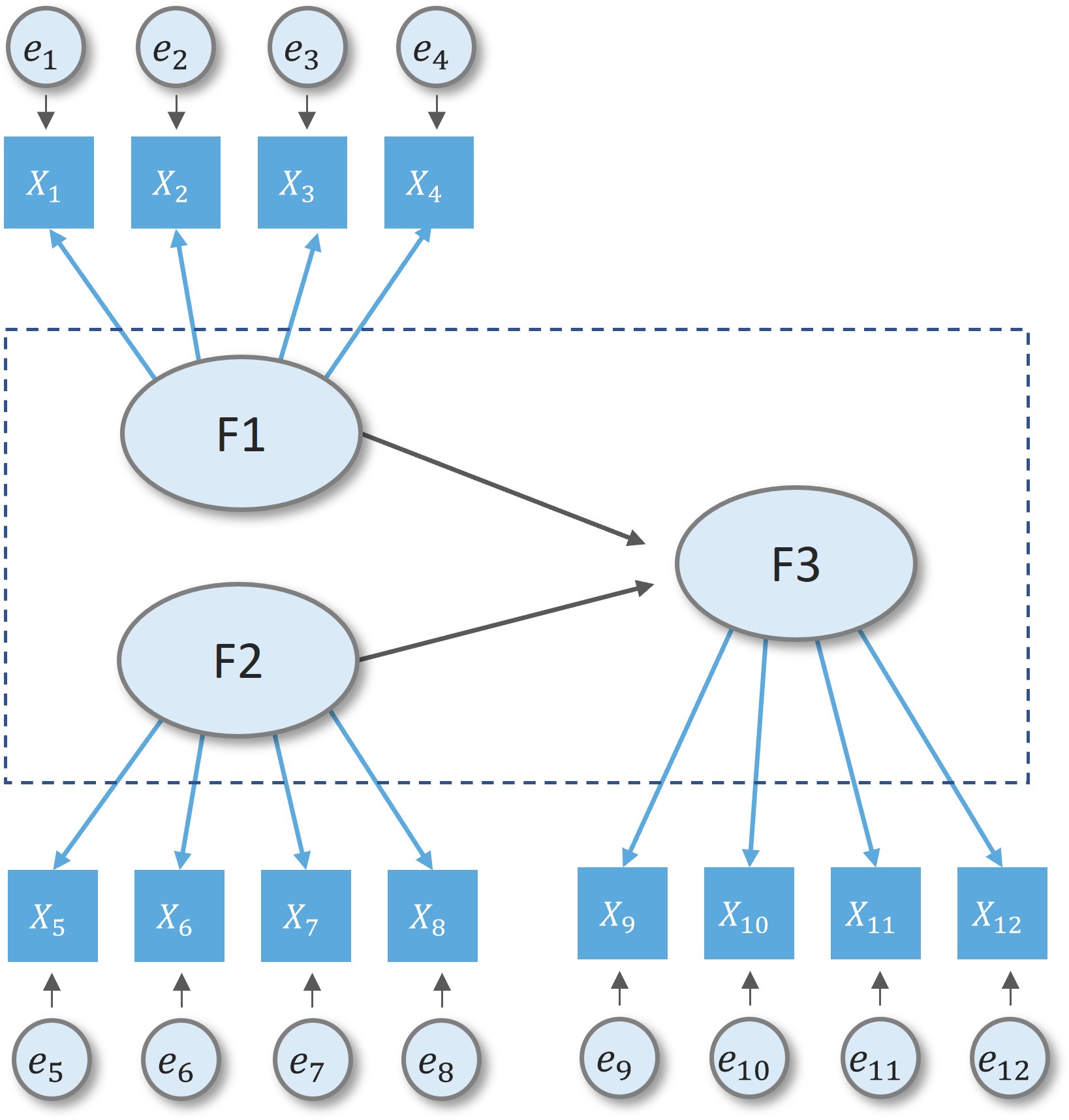
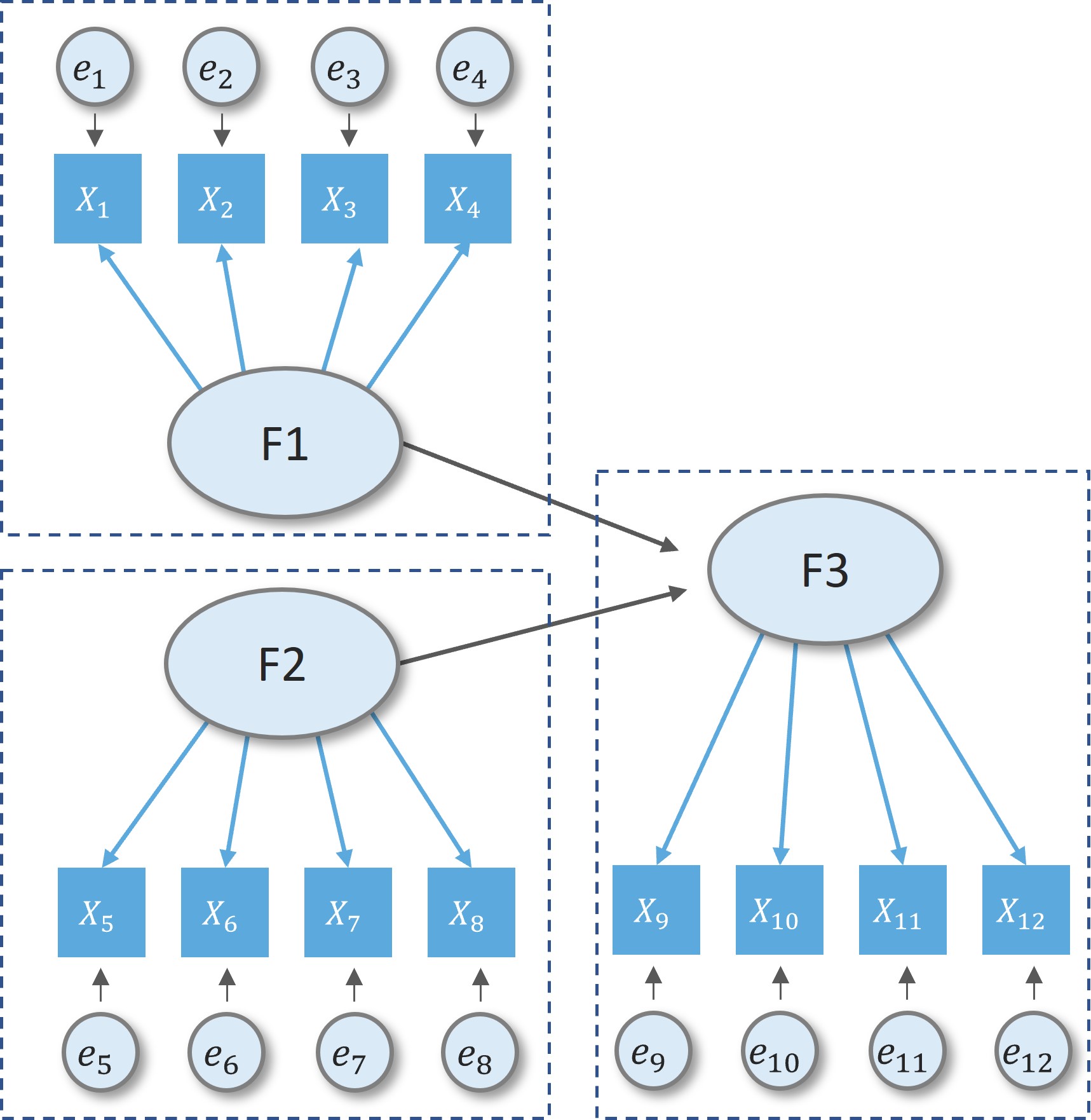
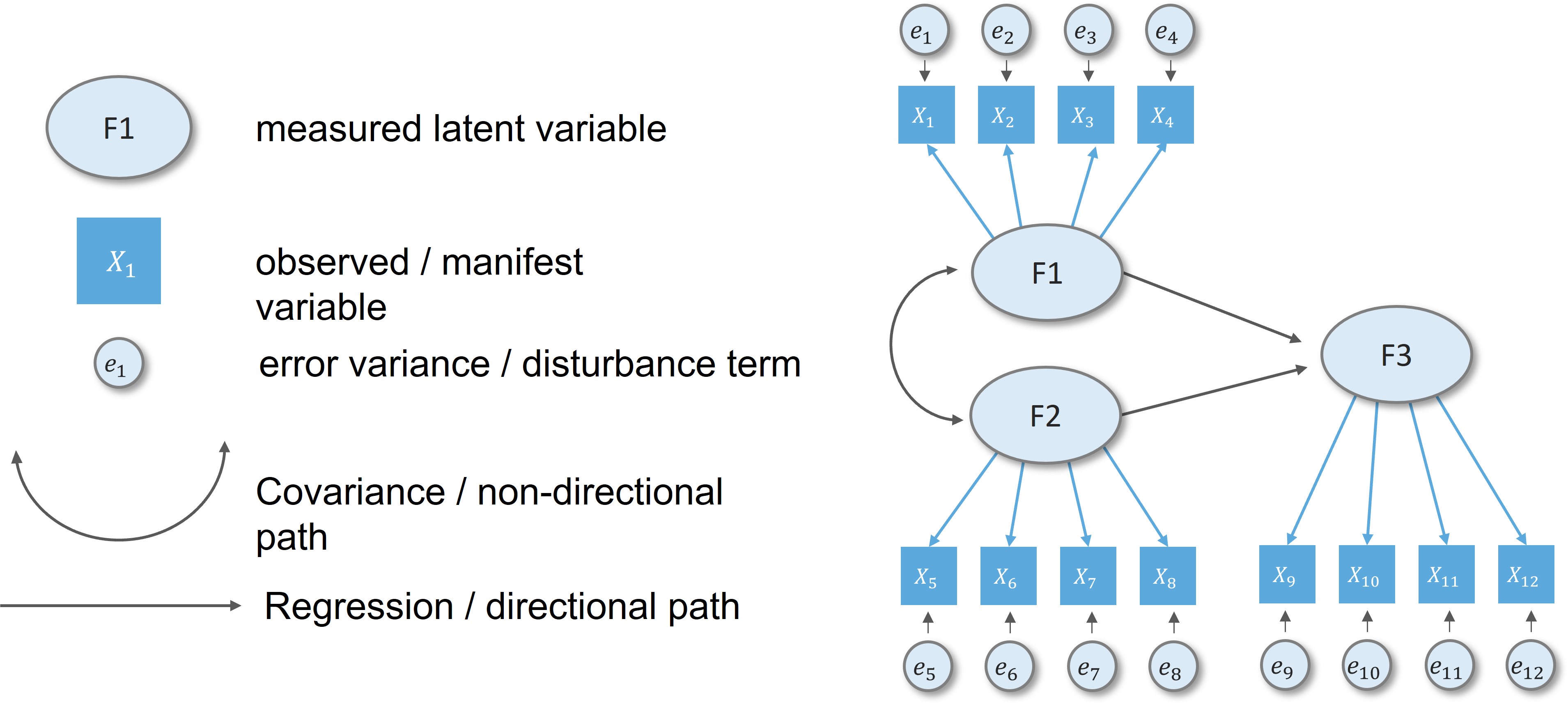
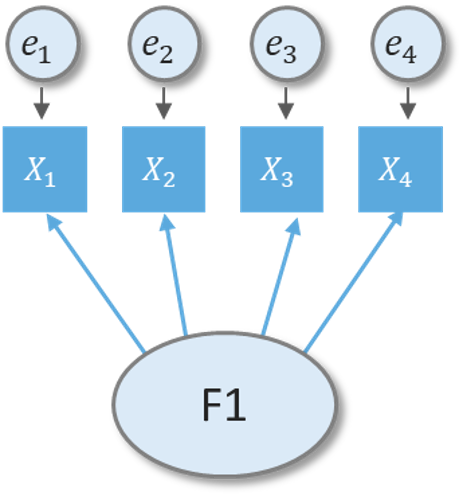
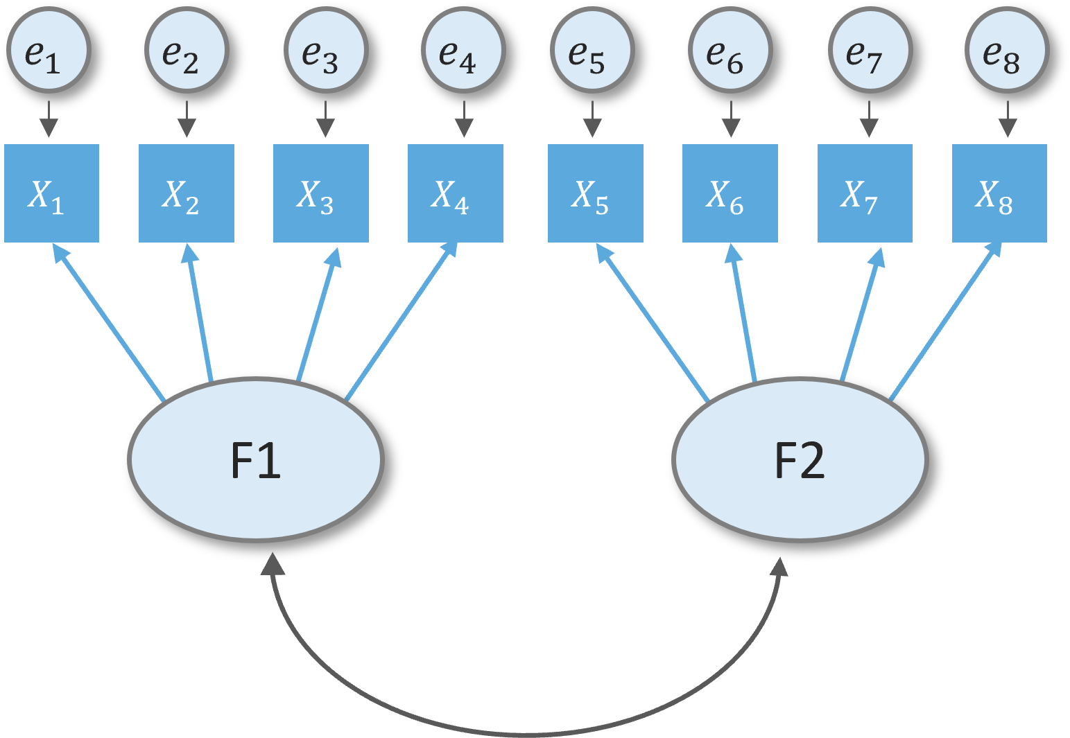
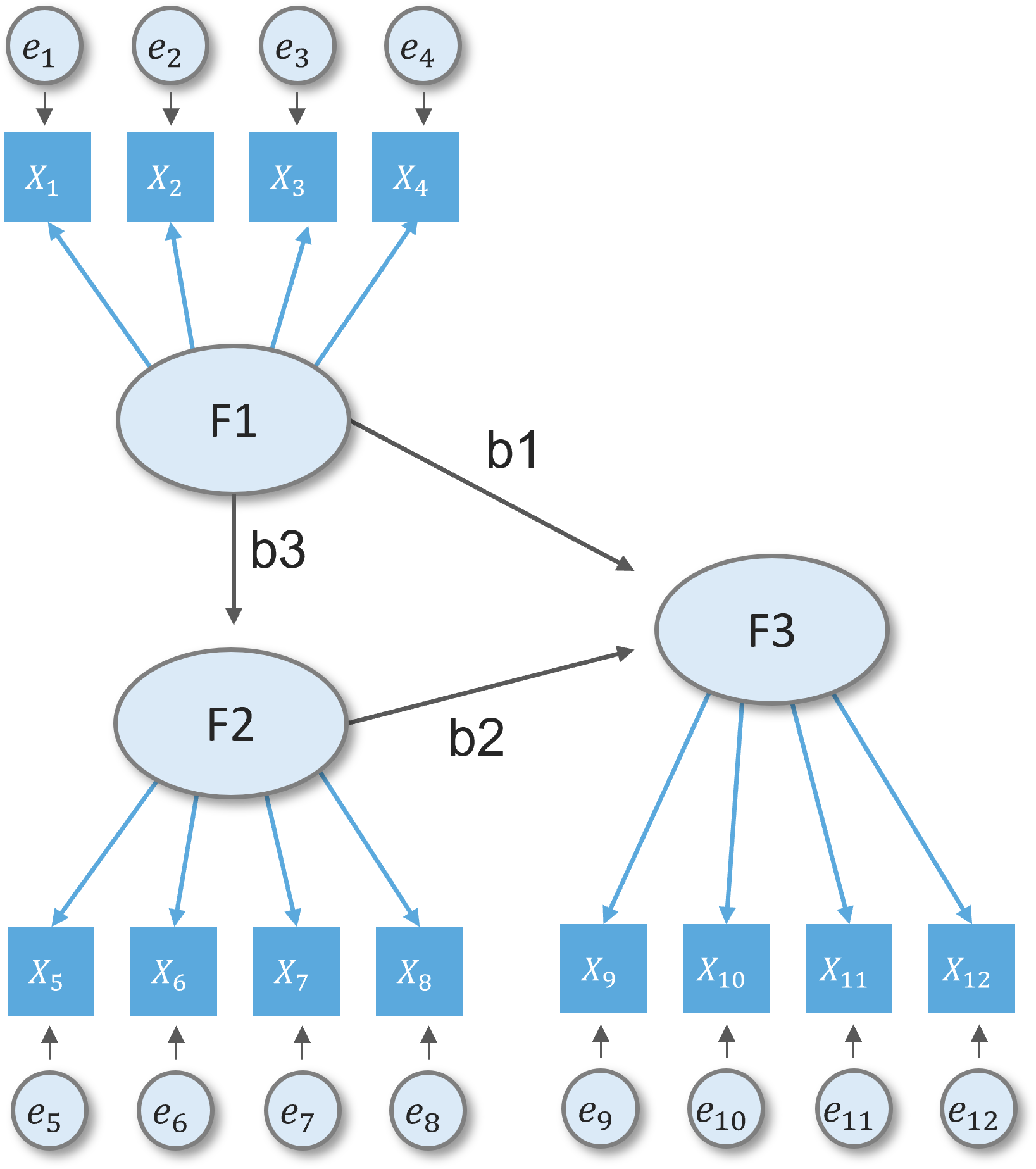
Basic SEM conventions
2. CFA-SEM with Lavaan R package
What is Lavaan?
“developed to provide useRs, researchers, and teachers a free open-source, but commercial quality”, Yves Rosseel (2012)
Check-out this lavaan tutorial
library(lavaan)
example(cfa)

cfa> ## The famous Holzinger and Swineford (1939) example
cfa> HS.model <- ' visual  =~ x1 + x2 + x3
cfa+               textual =~ x4 + x5 + x6
cfa+               speed   =~ x7 + x8 + x9 '

cfa> fit <- cfa(HS.model, data = HolzingerSwineford1939)

cfa> summary(fit, fit.measures = TRUE)
lavaan 0.6.13 ended normally after 35 iterations

  Estimator                                         ML
  Optimization method                           NLMINB
  Number of model parameters                        21

  Number of observations                           301

Model Test User Model:

  Test statistic                                85.306
  Degrees of freedom                                24
  P-value (Chi-square)                           0.000

Model Test Baseline Model:

  Test statistic                               918.852
  Degrees of freedom                                36
  P-value                                        0.000

User Model versus Baseline Model:

  Comparative Fit Index (CFI)                    0.931
  Tucker-Lewis Index (TLI)                       0.896

Loglikelihood and Information Criteria:

  Loglikelihood user model (H0)              -3737.745
  Loglikelihood unrestricted model (H1)      -3695.092

  Akaike (AIC)                                7517.490
  Bayesian (BIC)                              7595.339
  Sample-size adjusted Bayesian (SABIC)       7528.739

Root Mean Square Error of Approximation:

  RMSEA                                          0.092
  90 Percent confidence interval - lower         0.071
  90 Percent confidence interval - upper         0.114
  P-value H_0: RMSEA <= 0.050                    0.001
  P-value H_0: RMSEA >= 0.080                    0.840

Standardized Root Mean Square Residual:

  SRMR                                           0.065

Parameter Estimates:

  Standard errors                             Standard
  Information                                 Expected
  Information saturated (h1) model          Structured

Latent Variables:
                   Estimate  Std.Err  z-value  P(>|z|)
  visual =~
    x1                1.000
    x2                0.554    0.100    5.554    0.000
    x3                0.729    0.109    6.685    0.000
  textual =~
    x4                1.000
    x5                1.113    0.065   17.014    0.000
    x6                0.926    0.055   16.703    0.000
  speed =~
    x7                1.000
    x8                1.180    0.165    7.152    0.000
    x9                1.082    0.151    7.155    0.000

Covariances:
                   Estimate  Std.Err  z-value  P(>|z|)
  visual ~~
    textual           0.408    0.074    5.552    0.000
    speed             0.262    0.056    4.660    0.000
  textual ~~
    speed             0.173    0.049    3.518    0.000

Variances:
                   Estimate  Std.Err  z-value  P(>|z|)
   .x1                0.549    0.114    4.833    0.000
   .x2                1.134    0.102   11.146    0.000
   .x3                0.844    0.091    9.317    0.000
   .x4                0.371    0.048    7.779    0.000
   .x5                0.446    0.058    7.642    0.000
   .x6                0.356    0.043    8.277    0.000
   .x7                0.799    0.081    9.823    0.000
   .x8                0.488    0.074    6.573    0.000
   .x9                0.566    0.071    8.003    0.000
    visual            0.809    0.145    5.564    0.000
    textual           0.979    0.112    8.737    0.000
    speed             0.384    0.086    4.451    0.000
Major operators of lavaan syntax
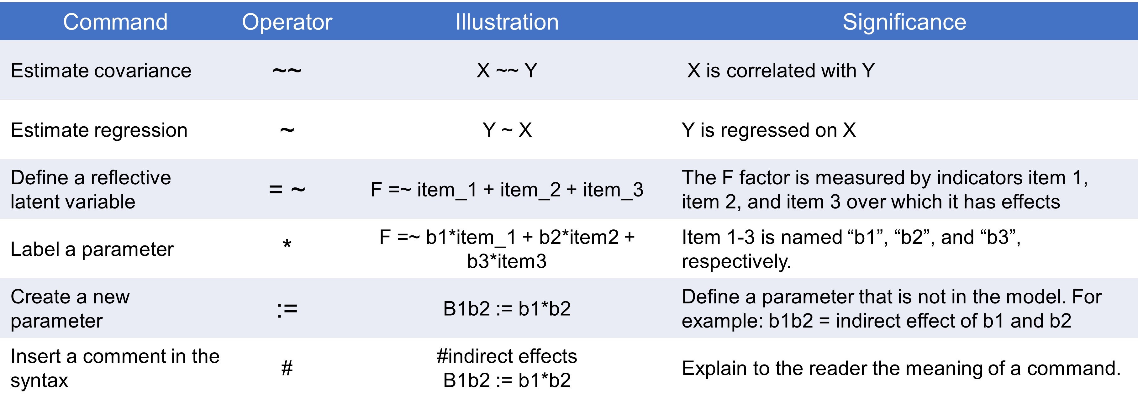
Major operators of lavaan syntax
Major operators of lavaan syntax
Major operators of lavaan syntax
Major operators of lavaan syntax
Major operators of lavaan syntax
Main steps in SEM
Defining constructs
Developing the overall measurement model
Assessing measurement model validity
Specifying the structural model
Assessing structural model validity
1. Defining Constructs
Dataset
HBAT company
HBAT is interested in understanding what affects employee’s attitudes and behaviors that contributes to employee’s retension.
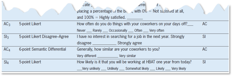
Defining individual constructs
Based on literature and preliminary interviews, a study was designed focusing on five key constructs.
Job satisfaction (JS) : reactions resulting from an appraisal of one’s job situation.
Organizational commitment (OC): extent to which an employees indentifies and feels part of HBAT.
Staying intention (SI): extent to which an employee intends to continue working for HBAT.
Environmental perceptions (EP): beliefs an employee has about day-to-day, physical working conditions.
Attitudes towards cowrokers (AC): attitudes an employee has toward the coworkers he/she interacts with on a regular basis.
Defining individual constructs

Step 2. Developing overall measurement model
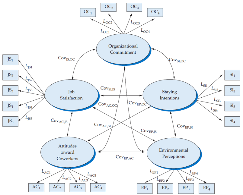
Developing overall measurement model
Measurement theory model (CFA) for HBAT employees
Direction of the relationship between factors is not yet defined.
Focus on confirming the specified model with empirical model (using empirical data), hence confirmatory.
Let’s practice!
Step 3. Assessing measurement model validity
Basic principles
Compare covariance matrix of the research data \(\text{S}\) and reproduced covariance \(\Sigma\)
Hypothesis:
Null: \(\text{S} = \Sigma\)
Atternative: \(\text{S} \ne \Sigma\)
Idea is to arrived with a parameter that minimizes the difference of \(\text{S}\) and \(\Sigma\)
cfa_fit <- cfa(cfa_model, data = hbat_data)
cfa_fit %>% summary()
lavaan 0.6.13 ended normally after 54 iterations
Estimator ML
Optimization method NLMINB
Number of model parameters 52
Number of observations 400
Model Test User Model:
Test statistic 240.738
Degrees of freedom 179
P-value (Chi-square) 0.001
Parameter Estimates:
Standard errors Standard
Information Expected
Information saturated (h1) model Structured
Latent Variables:
Estimate Std.Err z-value P(>|z|)
SI =~
SI1 1.000
SI2 1.073 0.055 19.563 0.000
SI3 1.065 0.066 16.053 0.000
SI4 1.167 0.061 19.230 0.000
JS =~
JS1 1.000
JS2 1.033 0.075 13.683 0.000
JS3 0.902 0.072 12.516 0.000
JS4 0.910 0.070 12.958 0.000
JS5 15.190 1.132 13.414 0.000
AC =~
AC1 1.000
AC2 1.236 0.067 18.392 0.000
AC3 1.037 0.055 18.870 0.000
AC4 1.146 0.063 18.255 0.000
EP =~
EP1 1.000
EP2 1.033 0.073 14.083 0.000
EP3 0.821 0.060 13.734 0.000
EP4 0.914 0.064 14.335 0.000
OC =~
OC1 1.000
OC2 1.314 0.108 12.209 0.000
OC3 0.783 0.076 10.322 0.000
OC4 1.165 0.097 11.968 0.000
Covariances:
Estimate Std.Err z-value P(>|z|)
SI ~~
JS 0.161 0.042 3.834 0.000
AC 0.249 0.048 5.161 0.000
EP 0.502 0.065 7.733 0.000
OC 0.574 0.080 7.191 0.000
JS ~~
AC 0.057 0.065 0.868 0.386
EP 0.303 0.078 3.892 0.000
OC 0.304 0.090 3.390 0.001
AC ~~
EP 0.372 0.088 4.251 0.000
OC 0.517 0.107 4.842 0.000
EP ~~
OC 0.925 0.143 6.469 0.000
Variances:
Estimate Std.Err z-value P(>|z|)
.SI1 0.258 0.023 11.121 0.000
.SI2 0.195 0.021 9.479 0.000
.SI3 0.464 0.038 12.264 0.000
.SI4 0.256 0.026 9.952 0.000
.JS1 0.807 0.074 10.960 0.000
.JS2 0.825 0.076 10.822 0.000
.JS3 0.930 0.078 11.910 0.000
.JS4 0.824 0.071 11.570 0.000
.JS5 196.867 17.681 11.135 0.000
.AC1 0.628 0.059 10.566 0.000
.AC2 0.973 0.092 10.617 0.000
.AC3 0.601 0.059 10.114 0.000
.AC4 0.867 0.081 10.742 0.000
.EP1 1.744 0.143 12.222 0.000
.EP2 0.937 0.091 10.245 0.000
.EP3 0.699 0.064 10.860 0.000
.EP4 0.637 0.066 9.659 0.000
.OC1 4.196 0.318 13.177 0.000
.OC2 1.029 0.149 6.929 0.000
.OC3 1.745 0.137 12.700 0.000
.OC4 1.267 0.138 9.193 0.000
SI 0.498 0.052 9.526 0.000
JS 0.981 0.122 8.038 0.000
AC 1.309 0.135 9.664 0.000
EP 1.600 0.214 7.471 0.000
OC 2.164 0.357 6.058 0.000Basic principles
Compare covariance matrix of the research data \(\text{S}\) and reproduced covariance \(\Sigma\)
Hypothesis:
Null: \(\text{S} = \Sigma\)
Atternative: \(\text{S} \ne \Sigma\)
Idea is to arrived with a parameter that minimizes the difference of \(\text{S}\) and \(\Sigma\)

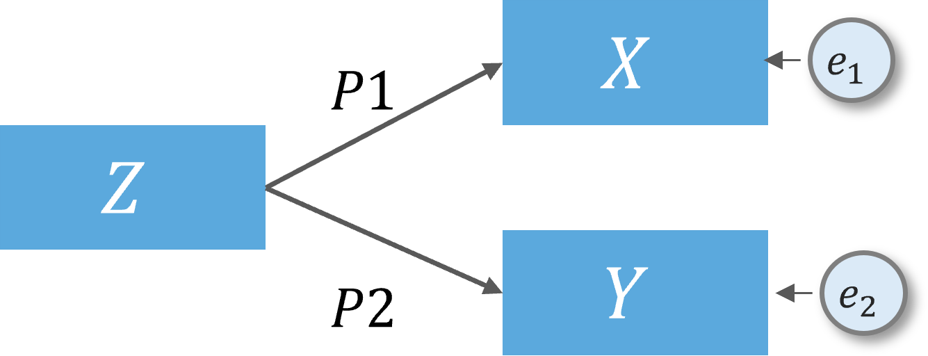
Basic principles
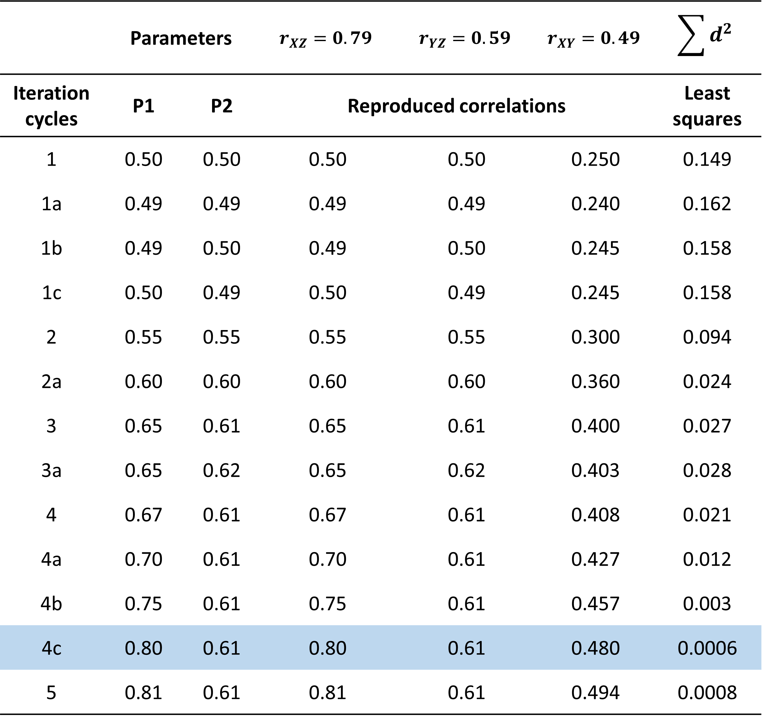
To understand the SEM process, consider the Table on the right.
e.g., iterative procedure using least square method.
Summary output
Overall results
Loadings
Variances
cfa_fit <- cfa(cfa_model, data = hbat_data)
summary(cfa_fit)
lavaan 0.6.13 ended normally after 54 iterations
Estimator ML
Optimization method NLMINB
Number of model parameters 52
Number of observations 400
Model Test User Model:
Test statistic 240.738
Degrees of freedom 179
P-value (Chi-square) 0.001
Parameter Estimates:
Standard errors Standard
Information Expected
Information saturated (h1) model Structured
Latent Variables:
Estimate Std.Err z-value P(>|z|)
SI =~
SI1 1.000
SI2 1.073 0.055 19.563 0.000
SI3 1.065 0.066 16.053 0.000
SI4 1.167 0.061 19.230 0.000
JS =~
JS1 1.000
JS2 1.033 0.075 13.683 0.000
JS3 0.902 0.072 12.516 0.000
JS4 0.910 0.070 12.958 0.000
JS5 15.190 1.132 13.414 0.000
AC =~
AC1 1.000
AC2 1.236 0.067 18.392 0.000
AC3 1.037 0.055 18.870 0.000
AC4 1.146 0.063 18.255 0.000
EP =~
EP1 1.000
EP2 1.033 0.073 14.083 0.000
EP3 0.821 0.060 13.734 0.000
EP4 0.914 0.064 14.335 0.000
OC =~
OC1 1.000
OC2 1.314 0.108 12.209 0.000
OC3 0.783 0.076 10.322 0.000
OC4 1.165 0.097 11.968 0.000
Covariances:
Estimate Std.Err z-value P(>|z|)
SI ~~
JS 0.161 0.042 3.834 0.000
AC 0.249 0.048 5.161 0.000
EP 0.502 0.065 7.733 0.000
OC 0.574 0.080 7.191 0.000
JS ~~
AC 0.057 0.065 0.868 0.386
EP 0.303 0.078 3.892 0.000
OC 0.304 0.090 3.390 0.001
AC ~~
EP 0.372 0.088 4.251 0.000
OC 0.517 0.107 4.842 0.000
EP ~~
OC 0.925 0.143 6.469 0.000
Variances:
Estimate Std.Err z-value P(>|z|)
.SI1 0.258 0.023 11.121 0.000
.SI2 0.195 0.021 9.479 0.000
.SI3 0.464 0.038 12.264 0.000
.SI4 0.256 0.026 9.952 0.000
.JS1 0.807 0.074 10.960 0.000
.JS2 0.825 0.076 10.822 0.000
.JS3 0.930 0.078 11.910 0.000
.JS4 0.824 0.071 11.570 0.000
.JS5 196.867 17.681 11.135 0.000
.AC1 0.628 0.059 10.566 0.000
.AC2 0.973 0.092 10.617 0.000
.AC3 0.601 0.059 10.114 0.000
.AC4 0.867 0.081 10.742 0.000
.EP1 1.744 0.143 12.222 0.000
.EP2 0.937 0.091 10.245 0.000
.EP3 0.699 0.064 10.860 0.000
.EP4 0.637 0.066 9.659 0.000
.OC1 4.196 0.318 13.177 0.000
.OC2 1.029 0.149 6.929 0.000
.OC3 1.745 0.137 12.700 0.000
.OC4 1.267 0.138 9.193 0.000
SI 0.498 0.052 9.526 0.000
JS 0.981 0.122 8.038 0.000
AC 1.309 0.135 9.664 0.000
EP 1.600 0.214 7.471 0.000
OC 2.164 0.357 6.058 0.000Summary output
Overall results
Degrees of freedom (df)
- \(df = \frac{1}{2} p (p + 1) - k\)
- \(p\) = total observed variables
- \(k\) = total estimated parameters
Identification
- Include at least three manifest variables
- Create models with \(df > 0\)
cfa_fit <- cfa(cfa_model, data = hbat_data)
summary(cfa_fit)
lavaan 0.6.13 ended normally after 54 iterations

  Estimator                                         ML
  Optimization method                           NLMINB
  Number of model parameters                        52

  Number of observations                           400

Model Test User Model:

  Test statistic                               240.738
  Degrees of freedom                               179
  P-value (Chi-square)                           0.001

Parameter Estimates:

  Standard errors                             Standard
  Information                                 Expected
  Information saturated (h1) model          Structured

Latent Variables:
                   Estimate  Std.Err  z-value  P(>|z|)
  SI =~
    SI1               1.000
    SI2               1.073    0.055   19.563    0.000
    SI3               1.065    0.066   16.053    0.000
    SI4               1.167    0.061   19.230    0.000
  JS =~
    JS1               1.000
    JS2               1.033    0.075   13.683    0.000
    JS3               0.902    0.072   12.516    0.000
    JS4               0.910    0.070   12.958    0.000
    JS5              15.190    1.132   13.414    0.000
  AC =~
    AC1               1.000
    AC2               1.236    0.067   18.392    0.000
    AC3               1.037    0.055   18.870    0.000
    AC4               1.146    0.063   18.255    0.000
  EP =~
    EP1               1.000
    EP2               1.033    0.073   14.083    0.000
    EP3               0.821    0.060   13.734    0.000
    EP4               0.914    0.064   14.335    0.000
  OC =~
    OC1               1.000
    OC2               1.314    0.108   12.209    0.000
    OC3               0.783    0.076   10.322    0.000
    OC4               1.165    0.097   11.968    0.000

Covariances:
                   Estimate  Std.Err  z-value  P(>|z|)
  SI ~~
    JS                0.161    0.042    3.834    0.000
    AC                0.249    0.048    5.161    0.000
    EP                0.502    0.065    7.733    0.000
    OC                0.574    0.080    7.191    0.000
  JS ~~
    AC                0.057    0.065    0.868    0.386
    EP                0.303    0.078    3.892    0.000
    OC                0.304    0.090    3.390    0.001
  AC ~~
    EP                0.372    0.088    4.251    0.000
    OC                0.517    0.107    4.842    0.000
  EP ~~
    OC                0.925    0.143    6.469    0.000

Variances:
                   Estimate  Std.Err  z-value  P(>|z|)
   .SI1               0.258    0.023   11.121    0.000
   .SI2               0.195    0.021    9.479    0.000
   .SI3               0.464    0.038   12.264    0.000
   .SI4               0.256    0.026    9.952    0.000
   .JS1               0.807    0.074   10.960    0.000
   .JS2               0.825    0.076   10.822    0.000
   .JS3               0.930    0.078   11.910    0.000
   .JS4               0.824    0.071   11.570    0.000
   .JS5             196.867   17.681   11.135    0.000
   .AC1               0.628    0.059   10.566    0.000
   .AC2               0.973    0.092   10.617    0.000
   .AC3               0.601    0.059   10.114    0.000
   .AC4               0.867    0.081   10.742    0.000
   .EP1               1.744    0.143   12.222    0.000
   .EP2               0.937    0.091   10.245    0.000
   .EP3               0.699    0.064   10.860    0.000
   .EP4               0.637    0.066    9.659    0.000
   .OC1               4.196    0.318   13.177    0.000
   .OC2               1.029    0.149    6.929    0.000
   .OC3               1.745    0.137   12.700    0.000
   .OC4               1.267    0.138    9.193    0.000
    SI                0.498    0.052    9.526    0.000
    JS                0.981    0.122    8.038    0.000
    AC                1.309    0.135    9.664    0.000
    EP                1.600    0.214    7.471    0.000
    OC                2.164    0.357    6.058    0.000
Summary output
Loadings
- Measures the strength of the relationship between items and factor.
cfa_fit <- cfa(cfa_model, data = hbat_data)
summary(cfa_fit, standardized = TRUE)
lavaan 0.6.13 ended normally after 54 iterations
Estimator ML
Optimization method NLMINB
Number of model parameters 52
Number of observations 400
Model Test User Model:
Test statistic 240.738
Degrees of freedom 179
P-value (Chi-square) 0.001
Parameter Estimates:
Standard errors Standard
Information Expected
Information saturated (h1) model Structured
Latent Variables:
Estimate Std.Err z-value P(>|z|) Std.lv Std.all
SI =~
SI1 1.000 0.706 0.811
SI2 1.073 0.055 19.563 0.000 0.757 0.864
SI3 1.065 0.066 16.053 0.000 0.752 0.741
SI4 1.167 0.061 19.230 0.000 0.823 0.852
JS =~
JS1 1.000 0.991 0.741
JS2 1.033 0.075 13.683 0.000 1.023 0.748
JS3 0.902 0.072 12.516 0.000 0.894 0.680
JS4 0.910 0.070 12.958 0.000 0.902 0.705
JS5 15.190 1.132 13.414 0.000 15.046 0.731
AC =~
AC1 1.000 1.144 0.822
AC2 1.236 0.067 18.392 0.000 1.414 0.820
AC3 1.037 0.055 18.870 0.000 1.187 0.837
AC4 1.146 0.063 18.255 0.000 1.312 0.815
EP =~
EP1 1.000 1.265 0.692
EP2 1.033 0.073 14.083 0.000 1.307 0.803
EP3 0.821 0.060 13.734 0.000 1.038 0.779
EP4 0.914 0.064 14.335 0.000 1.156 0.823
OC =~
OC1 1.000 1.471 0.583
OC2 1.314 0.108 12.209 0.000 1.934 0.886
OC3 0.783 0.076 10.322 0.000 1.151 0.657
OC4 1.165 0.097 11.968 0.000 1.714 0.836
Covariances:
Estimate Std.Err z-value P(>|z|) Std.lv Std.all
SI ~~
JS 0.161 0.042 3.834 0.000 0.230 0.230
AC 0.249 0.048 5.161 0.000 0.309 0.309
EP 0.502 0.065 7.733 0.000 0.562 0.562
OC 0.574 0.080 7.191 0.000 0.553 0.553
JS ~~
AC 0.057 0.065 0.868 0.386 0.050 0.050
EP 0.303 0.078 3.892 0.000 0.242 0.242
OC 0.304 0.090 3.390 0.001 0.209 0.209
AC ~~
EP 0.372 0.088 4.251 0.000 0.257 0.257
OC 0.517 0.107 4.842 0.000 0.307 0.307
EP ~~
OC 0.925 0.143 6.469 0.000 0.497 0.497
Variances:
Estimate Std.Err z-value P(>|z|) Std.lv Std.all
.SI1 0.258 0.023 11.121 0.000 0.258 0.342
.SI2 0.195 0.021 9.479 0.000 0.195 0.253
.SI3 0.464 0.038 12.264 0.000 0.464 0.451
.SI4 0.256 0.026 9.952 0.000 0.256 0.274
.JS1 0.807 0.074 10.960 0.000 0.807 0.451
.JS2 0.825 0.076 10.822 0.000 0.825 0.441
.JS3 0.930 0.078 11.910 0.000 0.930 0.538
.JS4 0.824 0.071 11.570 0.000 0.824 0.503
.JS5 196.867 17.681 11.135 0.000 196.867 0.465
.AC1 0.628 0.059 10.566 0.000 0.628 0.324
.AC2 0.973 0.092 10.617 0.000 0.973 0.327
.AC3 0.601 0.059 10.114 0.000 0.601 0.299
.AC4 0.867 0.081 10.742 0.000 0.867 0.335
.EP1 1.744 0.143 12.222 0.000 1.744 0.522
.EP2 0.937 0.091 10.245 0.000 0.937 0.354
.EP3 0.699 0.064 10.860 0.000 0.699 0.393
.EP4 0.637 0.066 9.659 0.000 0.637 0.323
.OC1 4.196 0.318 13.177 0.000 4.196 0.660
.OC2 1.029 0.149 6.929 0.000 1.029 0.216
.OC3 1.745 0.137 12.700 0.000 1.745 0.568
.OC4 1.267 0.138 9.193 0.000 1.267 0.301
SI 0.498 0.052 9.526 0.000 1.000 1.000
JS 0.981 0.122 8.038 0.000 1.000 1.000
AC 1.309 0.135 9.664 0.000 1.000 1.000
EP 1.600 0.214 7.471 0.000 1.000 1.000
OC 2.164 0.357 6.058 0.000 1.000 1.000Summary output
Variances
Refer to unique variance that the factor unable to account for. Similar to error term in OLS, hence it is also term as error variance.
cfa_fit <- cfa(cfa_model, data = hbat_data)
summary(cfa_fit, standardized = TRUE)
lavaan 0.6.13 ended normally after 54 iterations

  Estimator                                         ML
  Optimization method                           NLMINB
  Number of model parameters                        52

  Number of observations                           400

Model Test User Model:

  Test statistic                               240.738
  Degrees of freedom                               179
  P-value (Chi-square)                           0.001

Parameter Estimates:

  Standard errors                             Standard
  Information                                 Expected
  Information saturated (h1) model          Structured

Latent Variables:
                   Estimate  Std.Err  z-value  P(>|z|)   Std.lv  Std.all
  SI =~
    SI1               1.000                               0.706    0.811
    SI2               1.073    0.055   19.563    0.000    0.757    0.864
    SI3               1.065    0.066   16.053    0.000    0.752    0.741
    SI4               1.167    0.061   19.230    0.000    0.823    0.852
  JS =~
    JS1               1.000                               0.991    0.741
    JS2               1.033    0.075   13.683    0.000    1.023    0.748
    JS3               0.902    0.072   12.516    0.000    0.894    0.680
    JS4               0.910    0.070   12.958    0.000    0.902    0.705
    JS5              15.190    1.132   13.414    0.000   15.046    0.731
  AC =~
    AC1               1.000                               1.144    0.822
    AC2               1.236    0.067   18.392    0.000    1.414    0.820
    AC3               1.037    0.055   18.870    0.000    1.187    0.837
    AC4               1.146    0.063   18.255    0.000    1.312    0.815
  EP =~
    EP1               1.000                               1.265    0.692
    EP2               1.033    0.073   14.083    0.000    1.307    0.803
    EP3               0.821    0.060   13.734    0.000    1.038    0.779
    EP4               0.914    0.064   14.335    0.000    1.156    0.823
  OC =~
    OC1               1.000                               1.471    0.583
    OC2               1.314    0.108   12.209    0.000    1.934    0.886
    OC3               0.783    0.076   10.322    0.000    1.151    0.657
    OC4               1.165    0.097   11.968    0.000    1.714    0.836

Covariances:
                   Estimate  Std.Err  z-value  P(>|z|)   Std.lv  Std.all
  SI ~~
    JS                0.161    0.042    3.834    0.000    0.230    0.230
    AC                0.249    0.048    5.161    0.000    0.309    0.309
    EP                0.502    0.065    7.733    0.000    0.562    0.562
    OC                0.574    0.080    7.191    0.000    0.553    0.553
  JS ~~
    AC                0.057    0.065    0.868    0.386    0.050    0.050
    EP                0.303    0.078    3.892    0.000    0.242    0.242
    OC                0.304    0.090    3.390    0.001    0.209    0.209
  AC ~~
    EP                0.372    0.088    4.251    0.000    0.257    0.257
    OC                0.517    0.107    4.842    0.000    0.307    0.307
  EP ~~
    OC                0.925    0.143    6.469    0.000    0.497    0.497

Variances:
                   Estimate  Std.Err  z-value  P(>|z|)   Std.lv  Std.all
   .SI1               0.258    0.023   11.121    0.000    0.258    0.342
   .SI2               0.195    0.021    9.479    0.000    0.195    0.253
   .SI3               0.464    0.038   12.264    0.000    0.464    0.451
   .SI4               0.256    0.026    9.952    0.000    0.256    0.274
   .JS1               0.807    0.074   10.960    0.000    0.807    0.451
   .JS2               0.825    0.076   10.822    0.000    0.825    0.441
   .JS3               0.930    0.078   11.910    0.000    0.930    0.538
   .JS4               0.824    0.071   11.570    0.000    0.824    0.503
   .JS5             196.867   17.681   11.135    0.000  196.867    0.465
   .AC1               0.628    0.059   10.566    0.000    0.628    0.324
   .AC2               0.973    0.092   10.617    0.000    0.973    0.327
   .AC3               0.601    0.059   10.114    0.000    0.601    0.299
   .AC4               0.867    0.081   10.742    0.000    0.867    0.335
   .EP1               1.744    0.143   12.222    0.000    1.744    0.522
   .EP2               0.937    0.091   10.245    0.000    0.937    0.354
   .EP3               0.699    0.064   10.860    0.000    0.699    0.393
   .EP4               0.637    0.066    9.659    0.000    0.637    0.323
   .OC1               4.196    0.318   13.177    0.000    4.196    0.660
   .OC2               1.029    0.149    6.929    0.000    1.029    0.216
   .OC3               1.745    0.137   12.700    0.000    1.745    0.568
   .OC4               1.267    0.138    9.193    0.000    1.267    0.301
    SI                0.498    0.052    9.526    0.000    1.000    1.000
    JS                0.981    0.122    8.038    0.000    1.000    1.000
    AC                1.309    0.135    9.664    0.000    1.000    1.000
    EP                1.600    0.214    7.471    0.000    1.000    1.000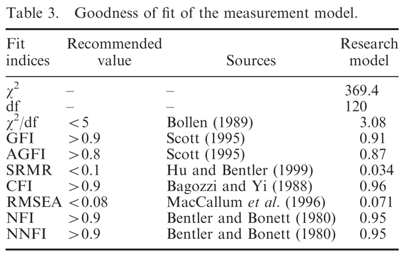
OC 2.164 0.357 6.058 0.000 1.000 1.000Fit indices
Goodness of fit indices
- Goodness-of-fit index (GFI)
- Adjusted goodness-fit-index (AGFI)
- Comparative fit index (CFI)
- Normed fit index (NFI)
- Non-normed fit index (NNF)
Badness of fit indices
- Standard root mean square of the residuals (SRMR)
- Root mean square error of approximation (RMSEA)
Fit indices
Goodness of fit indices
Goodness-of-fit index (GFI)
Adjusted goodness-fit-index (AGFI)
Comparative fit index (CFI)
Normed fit index (NFI)
Non-normed fit index (NNF)
fitMeasures(cfa_fit)
                 npar                  fmin                 chisq
               52.000                 0.301               240.738
                   df                pvalue        baseline.chisq
              179.000                 0.001              4452.567
          baseline.df       baseline.pvalue                   cfi
              210.000                 0.000                 0.985
                  tli                  nnfi                   rfi
                0.983                 0.983                 0.937
                  nfi                  pnfi                   ifi
                0.946                 0.806                 0.986
                  rni                  logl     unrestricted.logl
                0.985            -13916.782            -13796.413
                  aic                   bic                ntotal
            27937.564             28145.120               400.000
                 bic2                 rmsea        rmsea.ci.lower
            27980.120                 0.029                 0.019
       rmsea.ci.upper        rmsea.ci.level          rmsea.pvalue
                0.039                 0.900                 1.000
       rmsea.close.h0 rmsea.notclose.pvalue     rmsea.notclose.h0
                0.050                 0.000                 0.080
                  rmr            rmr_nomean                  srmr
                0.414                 0.414                 0.036
         srmr_bentler   srmr_bentler_nomean                  crmr
                0.036                 0.036                 0.037
          crmr_nomean            srmr_mplus     srmr_mplus_nomean
                0.037                 0.036                 0.036
                cn_05                 cn_01                   gfi
              351.949               376.401                 0.947
                 agfi                  pgfi                   mfi
                0.932                 0.734                 0.926
                 ecvi
                0.862
Fit indices
Goodness of fit indices
Goodness-of-fit index (GFI)
Adjusted goodness-fit-index (AGFI)
Comparative fit index (CFI)
Normed fit index (NFI)
Non-normed fit index (NNF)
Fit indices
Reliability and validity test
Reliability test
- Composite reliability
Validity test
Convergent validity
Discriminant validity
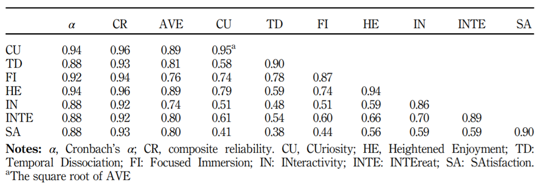
Reliability and validity test
Composite reliability:
alpha>0.70Convergent validity: AVE (
avevar) >0.50Discriminant validity:
omega>0.7
Let’s practice
Step 4: Specifying the structural model
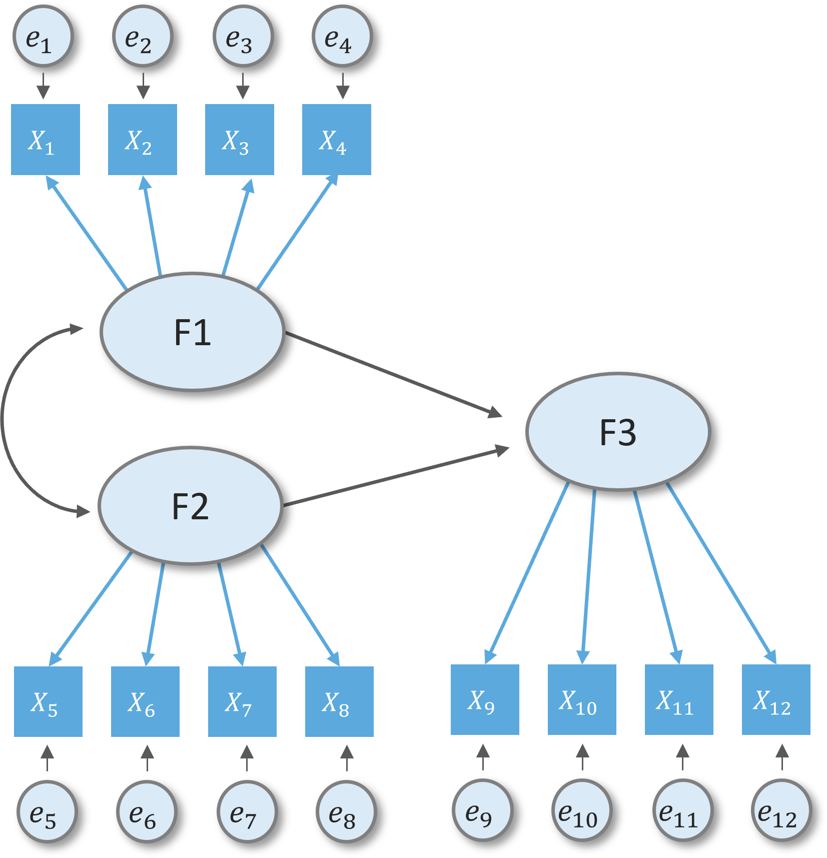
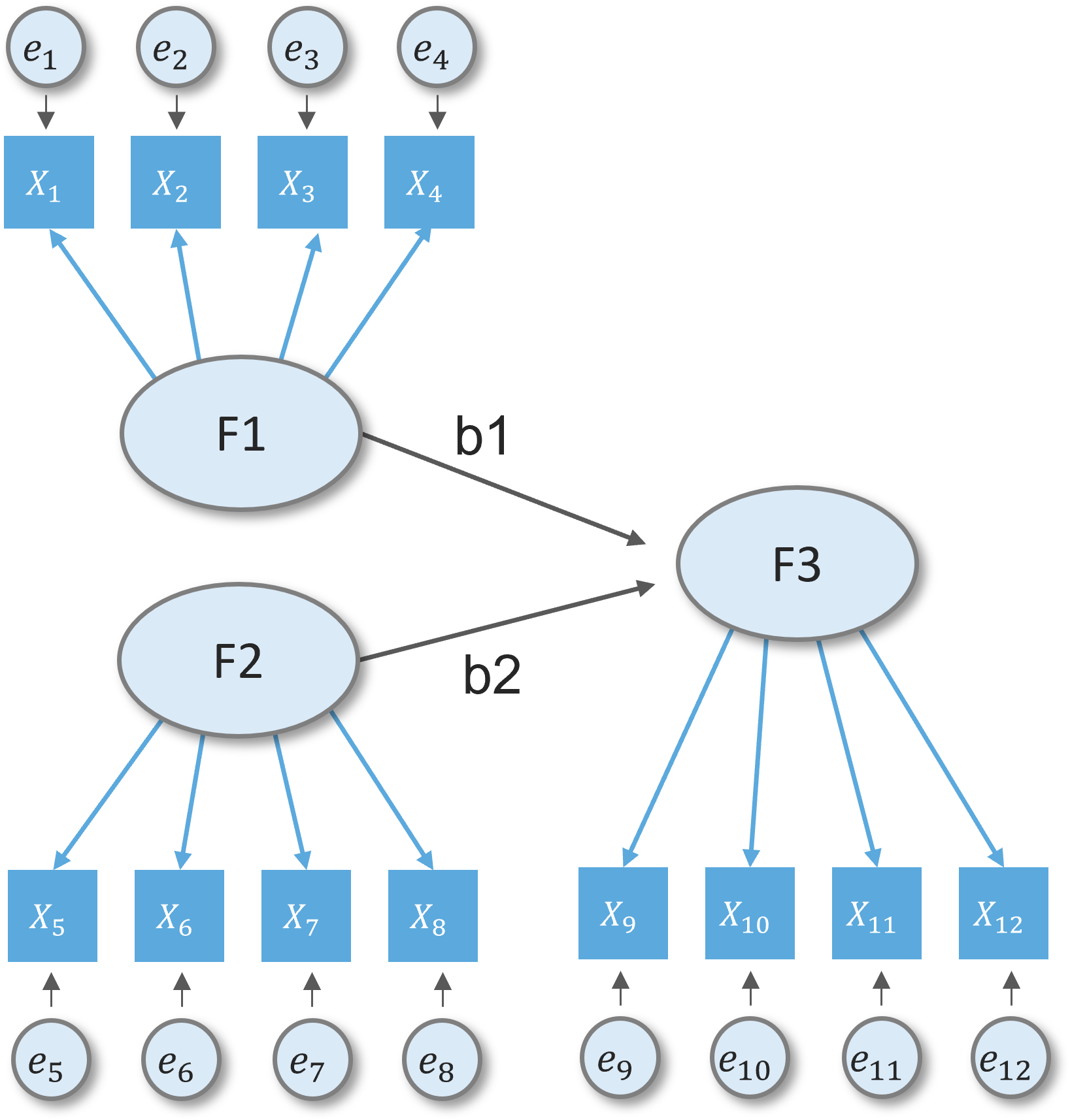
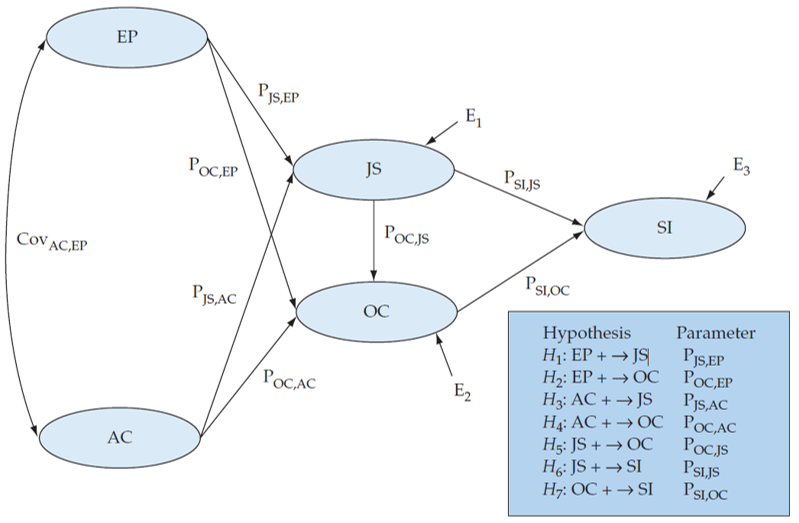
CFA model to structural model

Defining structural model
Hypotheses:
H1: Environmental perceptions are positively related to job satisfaction.
H2: Environmental perceptions are positively related to organizational commitment.
H3: Attitudes toward coworkers are positively related to job satisfaction.
H4: Attitudes toward coworkers are positively related to organizational commitment.
H5: Job satisfaction is related positively to organizational commitment.
H6: Job satisfaction is related positively to staying intentions.
H7: Organizational commitment is related positively to staying intention.
Defining structural model
Let’s practice
Defining structural model

Defining structural model

GOF measures between structural and CFA model
gof_indices <- c('chisq', 'df','pvalue', "gfi",
                 'rmsea', 'rmr', 'srmr', 'nfi',
                 'nnfi', 'cfi', 'agfi')
fitmeasures(sem_fit, fit.measures = gof_indices)
  chisq      df  pvalue     gfi   rmsea     rmr    srmr     nfi    nnfi     cfi
287.179 181.000   0.000   0.938   0.038   0.410   0.060   0.936   0.971   0.975
   agfi
  0.921
fitmeasures(cfa_fit, fit.measures = gof_indices)
  chisq      df  pvalue     gfi   rmsea     rmr    srmr     nfi    nnfi     cfi
240.738 179.000   0.001   0.947   0.029   0.414   0.036   0.946   0.983   0.985
   agfi
0.932 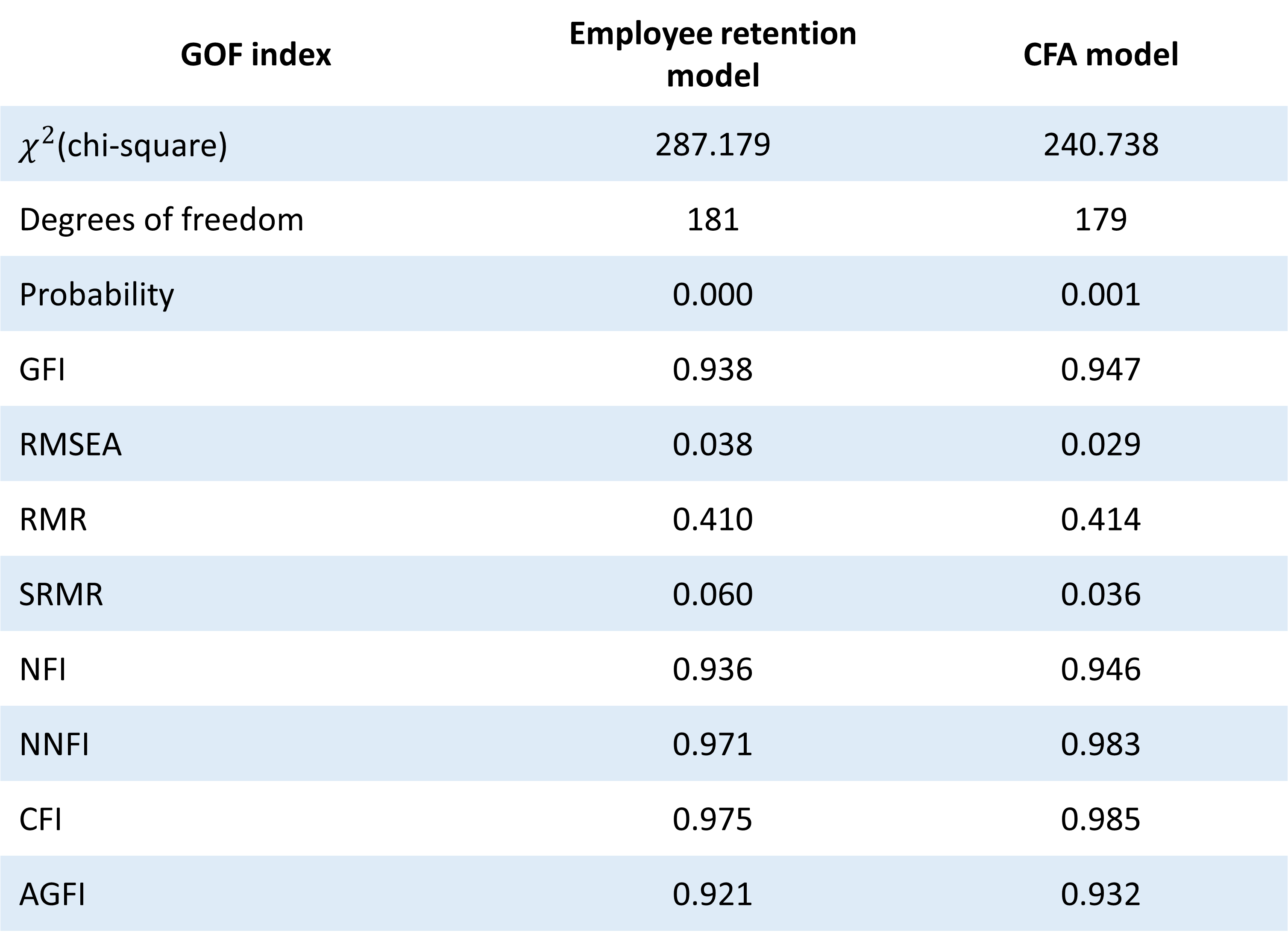
What’s next?
Modification indeces
Handling heywood cases
Comparing competing models
Formative scales in SEM
Higher-order factor analysis
Multigroup analysis

Thank you!

CFA & CB SEM