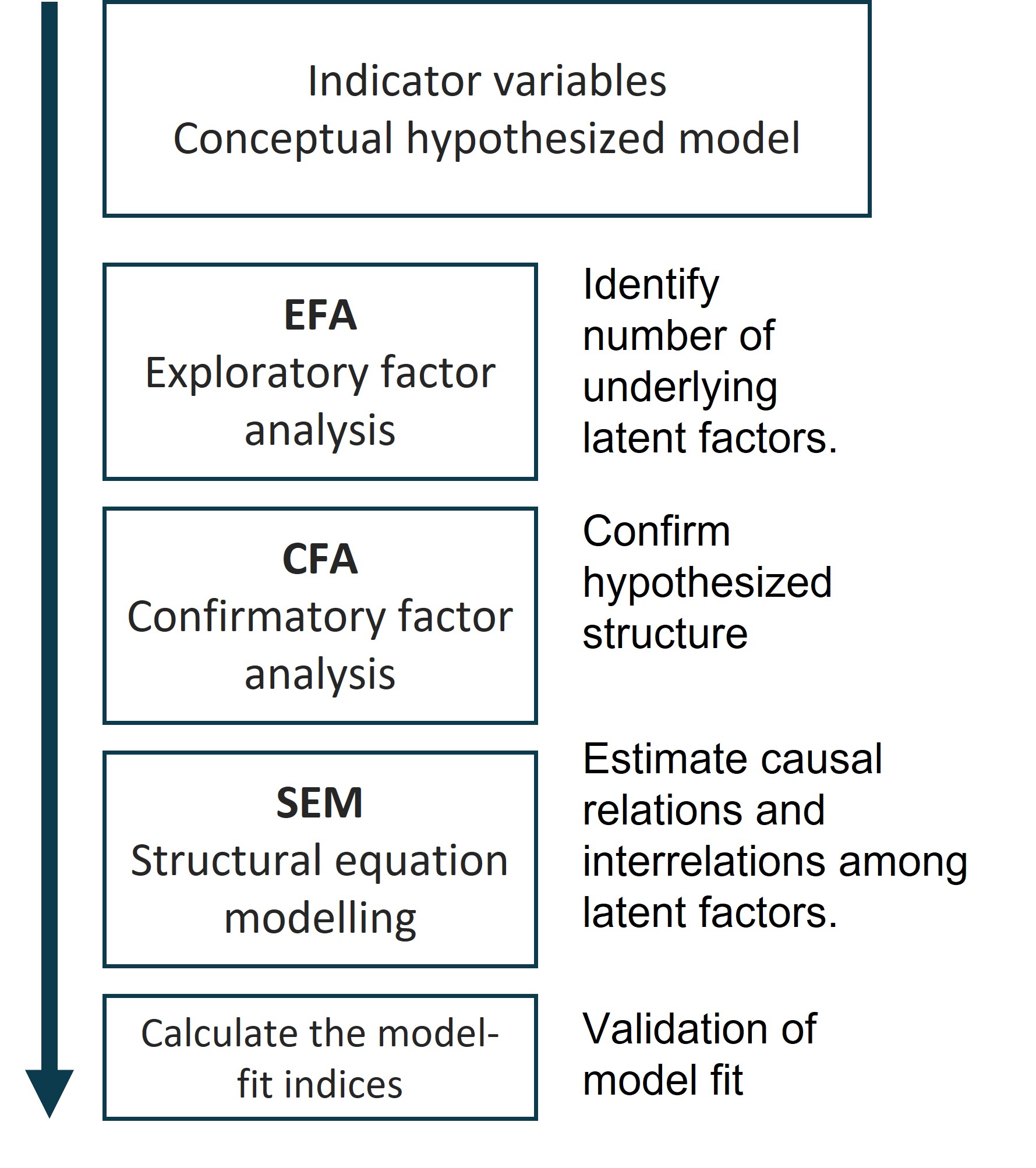
Training workshop on structural equation modelling (SEM) in R

Session 2: Exploratory Factor Analysis (EFA)

Factor analysis process

Stage 1: Objectives of factor analysis

Stage 2: Designing an Exploratory factor analysis

Stage 3: Assumptions in Exploratory factor analysis

Stage 4: Deriving factors and assessing overall fit

Stage 5: Interpreting the factors

Stage 1 : Objectives of factor analysis

Overview

Overview

Exploratory factor analysis

Exploratory or descriptive technique to determine the appropriate number of common factor.
No specifications are made in regards to the number of factors (initially) or the pattern of relationships between factor and indicators
Looking for patterns in the data

Confirmatory factor analysis

Should be conducted prior to the specifications of a structural model.
Researcher specifies the number of factors and the pattern of indicator-factor in advance.
Testing a theory that you know in advance

Stage 2: Designing an EFA

Variable selection and measurement issues

What types of variables can be used in factor analysis?

Primary requirement: a correlation value can be calculated among all variables.
e.g., metric variables, scale items, dummy variables to represent nonmetric variables.

How many variables or items should be used per factor?

Five or more per factor for scale development.
Three or more per factor for factor measurement (based on how degrees of freedom is computed).

Sample size

Some recommendations in literature:

Five cases minimum per estimated parameter (Bentler and Chou, 1987)
Monte carlo studies recommend 100 cases minimum and 200 is better for modest models (Loehlin, 2017)
Larger or complicated models, models with more latent variables or parameter estimates, require more cases.

Stage 3: Assumptions in EFA

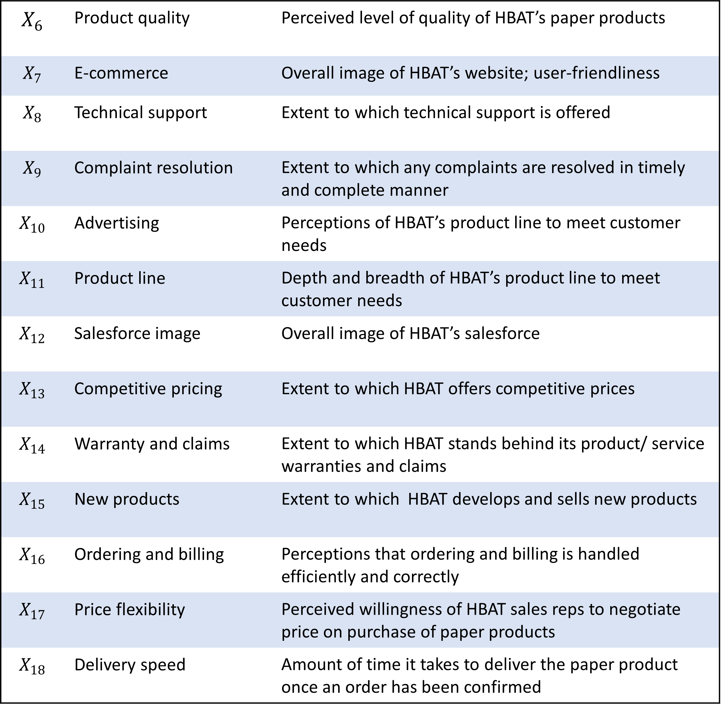
Sample Dataset

HBAT Industries, manufacturer of paper products.
Perceptions on a set of business functions.
Rating scale:
- 0 "poor" to 10 "excellent"

Sample Dataset

\(X_6\) product quality
\(X_7\) e-commerce
\(X_8\) technical support
\(X_9\) complaint resolution
\(X_{10}\) advertising
\(X_{11}\) product line
\(X_{12}\) salesforce image
\(X_{13}\) competitive pricing
\(X_{14}\) warranty claims
\(X_{15}\) packaging
\(X_{16}\) order & billing
\(X_{17}\) price flexibility
\(X_{18}\) delivery speed

Conceptual assumptions

Some uderlying structure does exist in the set of selected variables.
correlated variables and subsequent definition of factors do not guarantee relevance
- even if they meet the statistical requirement!
It is the responsibility of the researcher to ensure that observed patterns are conceptually valid and appropriate.

Determining appropriateness of EFA

Bartlett Test
Measure of Sampling Adequacy

Determining the appropriateness of EFA

1. Bartlett Test

Examines the entire correlation matrix
Test the hypothesis that correlation matrix is an identity matrix.
A significant result signifies data are appropriate for factor analysis.

library(EFAtools)
BARTLETT(data, N= nrow(data))

library(EFAtools)
BARTLETT(data, N= nrow(data))

✔ The Bartlett's test of sphericity was significant at an alpha level of .05.
  These data are probably suitable for factor analysis.

  𝜒²(55) = 619.27, p < .001

Determining the appropriateness of EFA

2. Kaiser-Meyen-Olkin (KMO Test)

Measure of sampling adequacy
Indicate the proportion of variance explained by the underlying factor.
Guidelines:
- \(\ge 0.90\) - marvelous
- \(\ge 0.80\) - meritorious
- \(\ge 0.70\) - middling
- \(\ge 0.60\) - mediocre
- \(\ge 0.50\) - miserable
- \(< 0.50\) - unacceptable

Determining the appropriateness of EFA

2. Kaiser-Meyen-Olkin (KMO Test)

library(psych)
KMO(data)

library(psych)
KMO(data)
Kaiser-Meyer-Olkin factor adequacy
Call: KMO(r = data)
Overall MSA =  0.65
MSA for each item = 
  x6   x7   x8   x9  x10  x11  x12  x13  x14  x16  x18 
0.51 0.63 0.52 0.79 0.78 0.62 0.62 0.75 0.51 0.76 0.67

Determining the appropriateness of EFA

2. Kaiser-Meyen-Olkin (KMO Test)

When overall MSA is less than 0.50
- Identify variables with lowest MSA subject for deletion.
- Recalculate MSA
- Repeat unitl overall MSA is 0.50 and above
Deletion of variables with MSA under 0.50 means variable’s correlation with
other variables are poorly representing the extracted factor.

Let’s practice!

Stage 4: Deriving factors and
assessing overall fit

Partitioning the variance of a variable

Unique variance

Variance associated with only a specific variable.
Not represented in the correlations among variables.
Specific variance
- associated uniquely with a single variable.
Error variance
- May be due to unreliability of data gathering process, measurement error, or a random component in the measured phenomenom.

Common variance

Shared variance with all other variables.
High common variance are more amenable for factor analysis.
Derived factors represents the shared or common variance among the variables.

Partitioning the variance of a variable

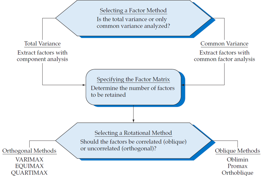
PCA vs Common factor analysis

Principal component analysis (PCA)

Considers the total variance
data reduction is a primary concern

Common factor analysis

Considers only the common variance or shared variance
Primary objective is to identify the latent dimensions or constructs

Exploring possible factors

1. Kaiser-Guttman Criterion

Only consider factors whose eigenvalues is greater than 1.
Rationale is that factor should account for the variance of at least a single variable if it is to be retained for interpretation.

library(EFAtools)
KGC(Data, eigen_type = "EFA")

Exploring possible factors

2. Scree test

Identify the optimum number of factors that can be extracted before the amount of unique variance begins to dominate the common variance.
Inflection point or the “elbow”

library(psych)
scree(data)

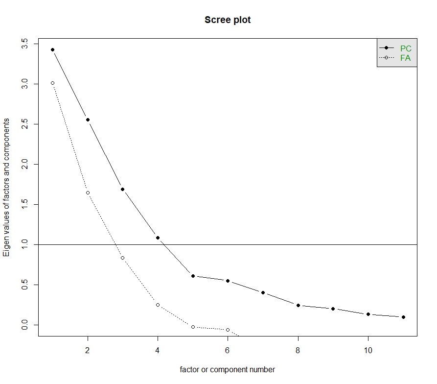
Exploring possible factors

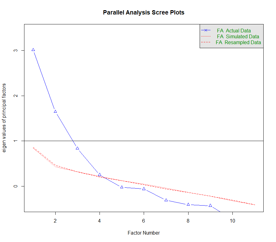
3. Parallel Test

Generates a large number of simulated dataset.
Each simulated dataset is factor analyzed.
- Results is the average eigenvalues across simulation.
- Values are then compared to the eigenvalues extracted from the original dataset.
- All factors with eigenvalues above those average eigenvalues are retained.

library(psych)
fa.parallel(data, fa = "fa")

Let’s practice!

Stage 5: Interpreting the factors

Three process of factor intepretation

1. Factor extraction

2. Factor rotation

3. Factor interpretation and re-specification

Factor extraction

fa_unrotated <- fa(r = data, nfactors = 4, rotate = "none")
print(fa_unrotated$loadings)

fa_unrotated <- fa(r = data, nfactors = 4, rotate = "none")
print(fa_unrotated$loadings)

Loadings:
    MR1    MR2    MR3    MR4   
x6   0.201 -0.408         0.463
x7   0.290  0.656  0.267  0.210
x8   0.278 -0.382  0.744 -0.169
x9   0.862        -0.255 -0.184
x10  0.287  0.456         0.127
x11  0.689 -0.454 -0.141  0.316
x12  0.398  0.807  0.348  0.255
x13 -0.231  0.553        -0.287
x14  0.378 -0.322  0.730 -0.151
x16  0.747        -0.176 -0.181
x18  0.895        -0.304 -0.198

                 MR1   MR2   MR3   MR4
SS loadings    3.215 2.226 1.500 0.679
Proportion Var 0.292 0.202 0.136 0.062
Cumulative Var 0.292 0.495 0.631 0.693

Loadings

Correlation of each variable and the factor.
Indicate the degree of correspondence between variable and factor.
Higher loadings making the variable representative of the factor.

Factor extraction

fa_unrotated <- fa(r = data, nfactors = 4,rotate = "none")
print(fa_unrotated$loadings)

fa_unrotated <- fa(r = data, nfactors = 4,rotate = "none")
print(fa_unrotated$loadings)

Loadings:
    MR1    MR2    MR3    MR4   
x6   0.201 -0.408         0.463
x7   0.290  0.656  0.267  0.210
x8   0.278 -0.382  0.744 -0.169
x9   0.862        -0.255 -0.184
x10  0.287  0.456         0.127
x11  0.689 -0.454 -0.141  0.316
x12  0.398  0.807  0.348  0.255
x13 -0.231  0.553        -0.287
x14  0.378 -0.322  0.730 -0.151
x16  0.747        -0.176 -0.181
x18  0.895        -0.304 -0.198

                 MR1   MR2   MR3   MR4
SS loadings    3.215 2.226 1.500 0.679
Proportion Var 0.292 0.202 0.136 0.062
Cumulative Var 0.292 0.495 0.631 0.693

Loadings

\(\le \pm 0.10 \approx\) zero
\(\pm 0.10\) to \(\pm 0.40\) meet the minimal level
\(\ge \pm 0.50\) practically significant
\(\ge \pm 0.70 \approx\) well-defined structure

SS loadings

Eigenvalues - column sum of squared factor loadings.
Relative importance of each factor in accounting for the variance associated with the set of variables.

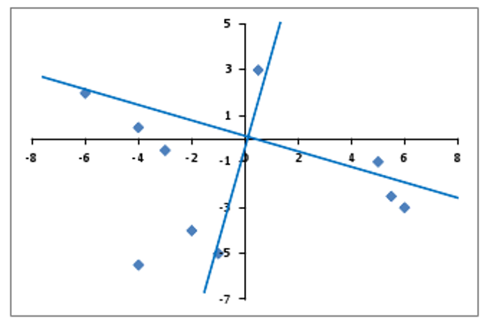
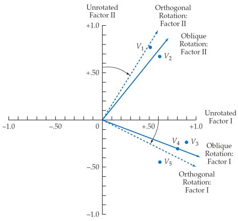
Factor rotation

Why do factor rotation?

To simplify the complexity of factor loadings.
Distribute the loading more clearly into the factors.
Facilitate interpretation.

Factor rotation

fa_rotated <- fa(r = data, nfactors = 4,rotate = "varimax")

par(mfrow = c(2, 1))
plot(fa_unrotated$loadings[,1],
     fa_unrotated$loadings[,2],
     xlab = "Factor 1",
     ylab = "Factor 2",
     ylim = c(-1, 1),
     xlim = c(-1, 1),
     main = "No rotation",
     pch = 19,
     cex = 2,
     col = "#6c757d") 
     abline(h=0, v=0)
     text(fa_unrotated$loadings[,1],
          fa_unrotated$loadings[,2],
          labels = rownames(fa_unrotated$loadings),
          pos = 4, cex = 1)

plot(fa_rotated$loadings[,1],
     fa_rotated$loadings[,2],
     xlab = "Factor 1",
     ylab = "Factor 2",
     ylim = c(-1, 1),
     xlim = c(-1, 1),
     main = "With rotation",
     pch = 19,
     cex = 2,
     col = "#6c757d")
     abline(h=0, v=0)
     text(fa_rotated$loadings[,1],
          fa_rotated$loadings[,2],
          labels = rownames(fa_unrotated$loadings),
          pos = 4, cex = 1)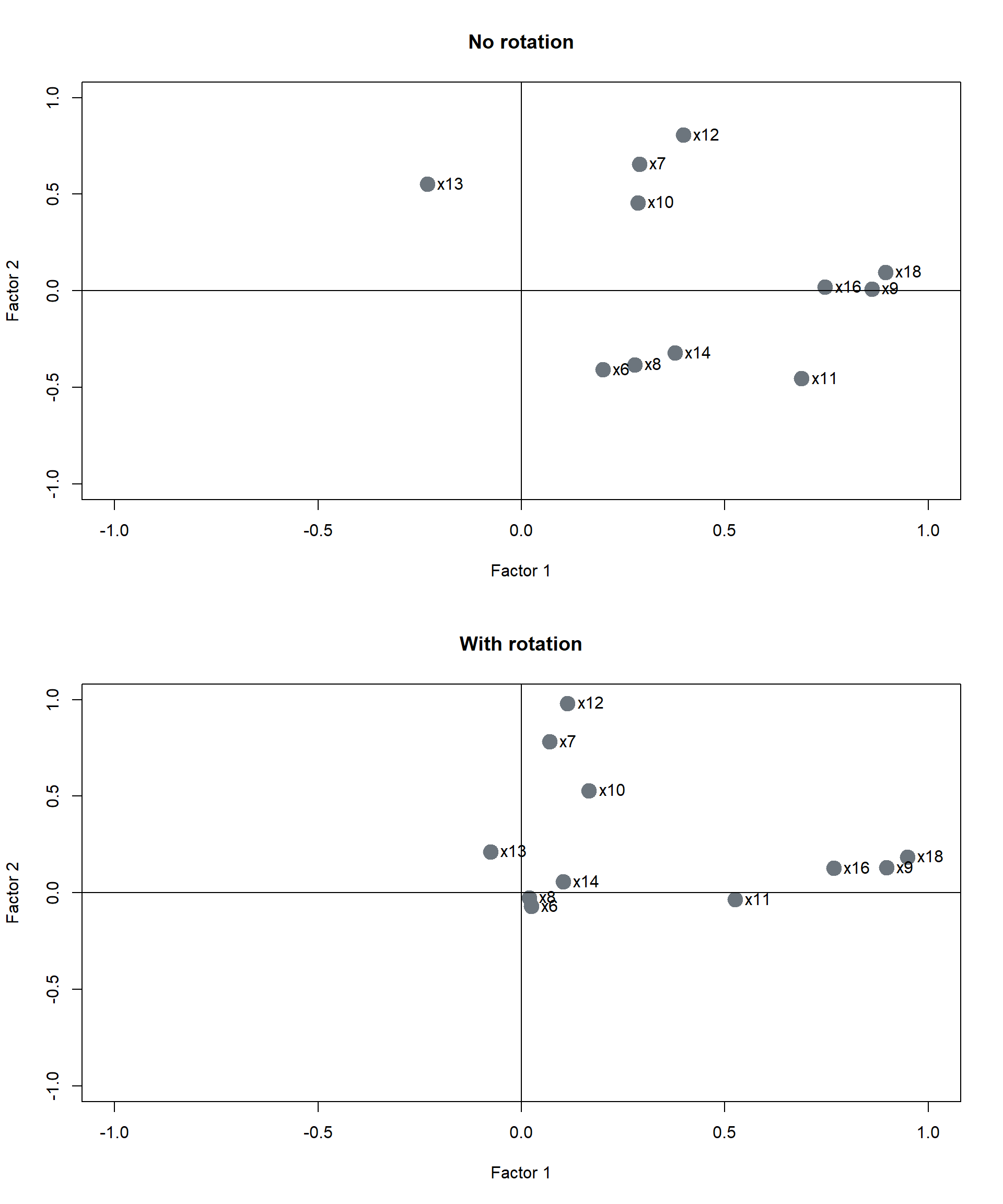

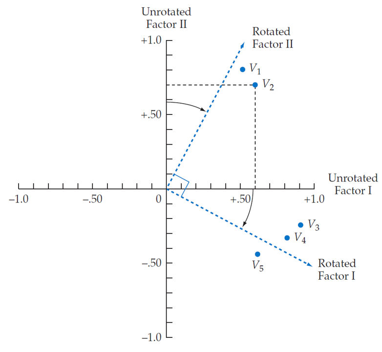
Factor rotation

Orthogonal rotation

axes are maintained at 90 degrees
orthogonal rotation methods
- Varimax - most commonly used
- Quartimax
- Equimax
Check-out some of these references
- IBM
- Factor analysis

Factor rotation

Orthogonal rotation

fa_varimax <- fa(r = data, nfactors = 4,rotate = "varimax")
fa_quartimax <- fa(r = data, nfactors = 4,rotate = "quartimax")
fa_equamax <- fa(r = data, nfactors = 4,rotate = "equamax")

par(mfrow = c(2, 2))

plot(fa_unrotated$loadings[,1],
     fa_unrotated$loadings[,2],
     xlab = "Factor 1",
     ylab = "Factor 2",
     ylim = c(-1, 1),
     xlim = c(-1, 1),
     main = "No rotation",
     cex.main = 3,
     pch = 19,
     cex = 4,
     col = "#6c757d") 
     abline(h=0, v=0)
     text(fa_unrotated$loadings[,1],
          fa_unrotated$loadings[,2],
          labels = rownames(fa_unrotated$loadings),
          pos = 4, cex = 2)
     
plot(fa_varimax$loadings[,1],
     fa_varimax$loadings[,2],
     xlab = "Factor 1",
     ylab = "Factor 2",
     ylim = c(-1, 1),
     xlim = c(-1, 1),
     main = "Varimax",
     cex.main = 3,
     pch = 19,
     cex = 4,
     col = "#6c757d") 
     abline(h=0, v=0)
     text(fa_varimax$loadings[,1],
          fa_varimax$loadings[,2],
          labels = rownames(fa_varimax$loadings),
          pos = 4, cex = 2)

plot(fa_quartimax$loadings[,1],
     fa_quartimax$loadings[,2],
     xlab = "Factor 1",
     ylab = "Factor 2",
     ylim = c(-1, 1),
     xlim = c(-1, 1),
     main = "Quartimax",
     cex.main = 3,
     pch = 19,
     cex = 4,
     col = "#6c757d") 
     abline(h=0, v=0)
     text(fa_quartimax$loadings[,1],
          fa_quartimax$loadings[,2],
          labels = rownames(fa_quartimax$loadings),
          pos = 4, cex = 2)
     
plot(fa_equamax$loadings[,1],
     fa_equamax$loadings[,2],
     xlab = "Factor 1",
     ylab = "Factor 2",
     ylim = c(-1, 1),
     xlim = c(-1, 1),
     main = "Equamax",
     cex.main = 3,
     pch = 19,
     cex = 4,
     col = "#6c757d") 
     abline(h=0, v=0)
     text(fa_equamax$loadings[,1],
          fa_equamax$loadings[,2],
          labels = rownames(fa_equamax$loadings),
          pos = 4, cex = 2)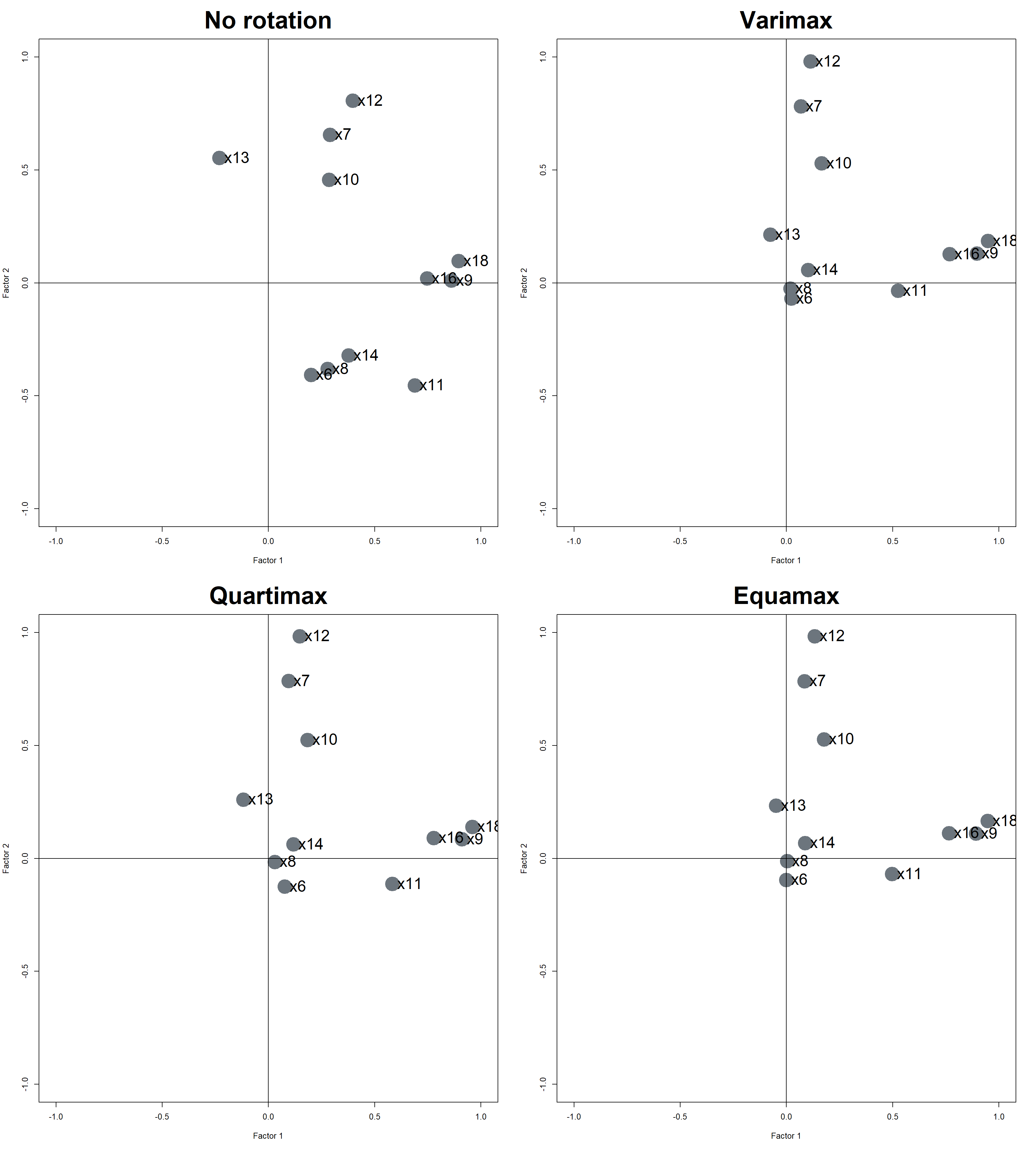

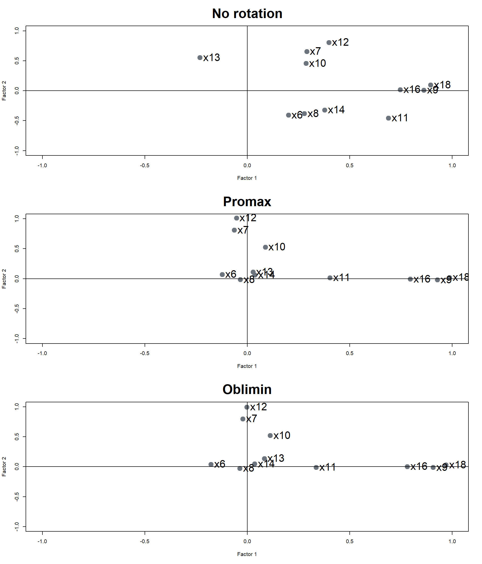
Factor rotation

Oblique rotation rotation

allow correlated factors
suited to the goal of theoretically meaningful constructs
oblique rotation methods
- Promax
- Oblimin

Factor rotation

Oblique rotation

fa_promax <- fa(r = data, nfactors = 4,rotate = "promax")
fa_oblimin <- fa(r = data, nfactors = 4,rotate = "oblimin")


par(mfrow = c(1, 3))

plot(fa_unrotated$loadings[,1],
     fa_unrotated$loadings[,2],
     xlab = "Factor 1",
     ylab = "Factor 2",
     ylim = c(-1, 1),
     xlim = c(-1, 1),
     main = "No rotation",
     pch = 19,
     col = "#6c757d") 
     abline(h=0, v=0)
     text(fa_unrotated$loadings[,1],
          fa_unrotated$loadings[,2],
          labels = rownames(fa_unrotated$loadings),
          pos = 4, cex = 0.5)
     
plot(fa_promax$loadings[,1],
     fa_promax$loadings[,2],
     xlab = "Factor 1",
     ylab = "Factor 2",
     ylim = c(-1, 1),
     xlim = c(-1, 1),
     main = "Promax",
     pch = 19,
     col = "#6c757d") 
     abline(h=0, v=0)
     text(fa_promax$loadings[,1],
          fa_promax$loadings[,2],
          labels = rownames(fa_promax$loadings),
          pos = 4, cex = 0.5)

plot(fa_oblimin$loadings[,1],
     fa_oblimin$loadings[,2],
     xlab = "Factor 1",
     ylab = "Factor 2",
     ylim = c(-1, 1),
     xlim = c(-1, 1),
     main = "Oblimin",
     pch = 19,
     col = "#6c757d") 
     abline(h=0, v=0)
     text(fa_oblimin$loadings[,1],
          fa_oblimin$loadings[,2],
          labels = rownames(fa_oblimin$loadings),
          pos = 4, cex = 0.5)

Factor interpretation and respecification

each variable has a high loadings on one factor only
each factor has a high loadings for only a subset of the items.

fa_varimax <- fa(r = data, nfactors = 4, rotate = "varimax")
print(fa_varimax$loadings, sort = TRUE)

fa_varimax <- fa(r = data, nfactors = 4, rotate = "varimax")
print(fa_varimax$loadings, sort = TRUE)

Loadings:
    MR1    MR2    MR3    MR4   
x9   0.897  0.130         0.132
x16  0.768  0.127              
x18  0.949  0.185              
x7          0.781        -0.115
x10  0.166  0.529              
x12  0.114  0.980        -0.133
x8                 0.890  0.115
x14  0.103         0.879  0.129
x6                        0.647
x11  0.525         0.127  0.712
x13         0.213 -0.209 -0.590

                 MR1   MR2   MR3   MR4
SS loadings    2.635 1.973 1.641 1.371
Proportion Var 0.240 0.179 0.149 0.125
Cumulative Var 0.240 0.419 0.568 0.693

Factor interpretation and respecification

each variable has a high loadings on one factor only
each factor has a high loadings for only a subset of the items.

fa_varimax <- fa(r = data, nfactors = 4, rotate = "varimax")
print(fa_varimax$loadings, sort = TRUE, cutoff = 0.4)

fa_varimax <- fa(r = data, nfactors = 4, rotate = "varimax")
print(fa_varimax$loadings, sort = TRUE, cutoff = 0.4)

Loadings:
    MR1    MR2    MR3    MR4   
x9   0.897                     
x16  0.768                     
x18  0.949                     
x7          0.781              
x10         0.529              
x12         0.980              
x8                 0.890       
x14                0.879       
x6                        0.647
x11  0.525                0.712
x13                      -0.590

                 MR1   MR2   MR3   MR4
SS loadings    2.635 1.973 1.641 1.371
Proportion Var 0.240 0.179 0.149 0.125
Cumulative Var 0.240 0.419 0.568 0.693

Factor interpretation and respecification

What to do with cross-loadings?

Ratio of variance (JF Hair et al. 2019)

1 to 1.5 - problematic
1.5 to 2.0 - potential cross-loading
2.0 and higher - ignorable

Example:

\(X_{11}\)
MR1: 0.525
MR2: 0.712
\(0.712^2 \div 0.525^2 = 1.8\)

fa_varimax <- fa(r = data, nfactors = 4, rotate = "varimax")
print(fa_varimax$loadings, sort = TRUE, cutoff = 0.4)

fa_varimax <- fa(r = data, nfactors = 4, rotate = "varimax")
print(fa_varimax$loadings, sort = TRUE, cutoff = 0.4)

Loadings:
    MR1    MR2    MR3    MR4   
x9   0.897                     
x16  0.768                     
x18  0.949                     
x7          0.781              
x10         0.529              
x12         0.980              
x8                 0.890       
x14                0.879       
x6                        0.647
x11  0.525                0.712
x13                      -0.590

                 MR1   MR2   MR3   MR4
SS loadings    2.635 1.973 1.641 1.371
Proportion Var 0.240 0.179 0.149 0.125
Cumulative Var 0.240 0.419 0.568 0.693

Factor interpretation and respecification

Naming of factors

MR1: Postsale customer service
- x9 Complaint resolutions
- x16 Order & Billing
- x18 Delivery speed
MR2: Marketing
- x7 E-Commerce
- x10 Advertising
- x12 Salesforce image

MR3: Technical support
- x8 Technical support
- x14 Warranty and claims
MR4: Product value
- x6 Product quality
- x11 Product line
- x13 Competitive pricing

Factor interpretation and respecification

Extracting factor scores

MR1: Postsale customer service
MR2: Marketing
MR3: Technical support
MR4: Product value

fa_varimax$scores %>% round(4) %>% data.frame() %>% tibble()

fa_varimax$scores %>% round(4) %>% data.frame() %>% tibble()
# A tibble: 100 × 4
      MR1    MR2    MR3     MR4
    <dbl>  <dbl>  <dbl>   <dbl>
 1 -0.139  0.940 -1.72   0.0968
 2  1.64  -2.04  -0.591  0.650 
 3  0.356  0.876  0.016  1.38  
 4 -1.22  -0.557  1.25  -0.646 
 5 -0.486 -0.421 -0.031  0.476 
 6 -0.592 -1.31  -1.20  -0.959 
 7 -2.54   0.417 -0.569 -1.30  
 8 -0.115 -0.118 -0.707 -1.36  
 9  0.952  0.372 -0.139 -0.929 
10  0.586  0.408 -0.462 -0.674 
# … with 90 more rows

Training workshop on structural equation modelling (SEM) in R

Factor analysis process

Stage 1 : Objectives of factor analysis

Overview

Overview

Exploratory factor analysis

Confirmatory factor analysis

Stage 2: Designing an EFA

Variable selection and measurement issues

Sample size

Stage 3: Assumptions in EFA

Sample Dataset

Sample Dataset

Conceptual assumptions

Determining appropriateness of EFA

Determining the appropriateness of EFA

1. Bartlett Test

Determining the appropriateness of EFA

2. Kaiser-Meyen-Olkin (KMO Test)

Determining the appropriateness of EFA

2. Kaiser-Meyen-Olkin (KMO Test)

Determining the appropriateness of EFA

2. Kaiser-Meyen-Olkin (KMO Test)

Let’s practice!

Stage 4: Deriving factors and assessing overall fit

Partitioning the variance of a variable

Unique variance

Common variance

Partitioning the variance of a variable

PCA vs Common factor analysis

Principal component analysis (PCA)

Common factor analysis

Exploring possible factors

1. Kaiser-Guttman Criterion

Exploring possible factors

2. Scree test

Exploring possible factors

3. Parallel Test

Let’s practice!

Stage 5: Interpreting the factors

Three process of factor intepretation

1. Factor extraction

2. Factor rotation

3. Factor interpretation and re-specification

Factor extraction

Loadings

Factor extraction

Loadings

SS loadings

Factor rotation

Why do factor rotation?

Factor rotation

Factor rotation

Orthogonal rotation

Factor rotation

Orthogonal rotation

Factor rotation

Oblique rotation rotation

Factor rotation

Oblique rotation

Factor interpretation and respecification

Factor interpretation and respecification

Factor interpretation and respecification

Factor interpretation and respecification

Naming of factors

Factor interpretation and respecification

Extracting factor scores

Let’s practice!

Thank you!

Stage 4: Deriving factors and
assessing overall fit